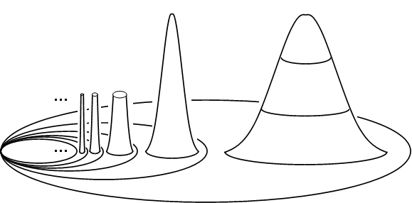
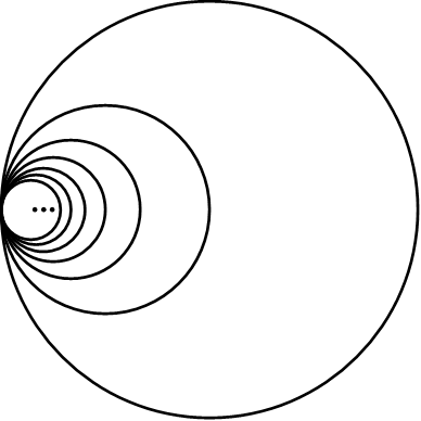
Here is one of my favorite spaces: The earring space, i.e. the “shrinking wedge of circles.”

The earring space
This space is the first step into the world of “wild” topological spaces. This post is meant to be an introduction into how one can understand the fundamental group of this space, which I will just refer to as the earring group. I’m no longer using “Hawaiian” on purpose. In fact, this is not just a regular group. If you can imagine groups (like the complex numbers) with geometrically relevant, natural infinite product operations, and is a “free” object of this type.
The earring space  is usually defined as the following planar set: let
  be the circle of radius
  centered at
  . Now take the union
  with the subspace topology of
  .
.
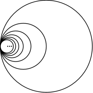
The key feature of this space is that if  is any open neighborhood of the “wild” point
  , then there is an
  such that
  for all
  . Note that the earring space has the same underlying set as the infinite wedge
  of circles, however the topology of is finer than that of . So there is a canonical continuous bijection
  , which is not a homeomorphism.
Topological facts: is a connected, one-dimensional, locally path connected, compact metric space.
Other ways to construct :
- As a one-point compactification:
 is homeomorphic to the one-point compactification of a countable disjoint union
  of open intervals.
- As a subspace of
 : View as a subspace of in the obvious way and give it the subspace topology. The resulting space is homeomorphic to .
- As an inverse limit: Let
 . If
. If  , there is a retraction
  which collapses the circles
  ,
,  to
to  . These maps form an inverse system
  . The inverse limit
  of this inverse system is homeormorphic to .
The really interesting things happen when you start considering loops and their homotopy classes, i.e. the fundamental group  . For each
  consider the loop
 ![\ell_n:[0,1]\to \mathbb{E}](https://s0.wp.com/latex.php?latex=%5Cell_n%3A%5B0%2C1%5D%5Cto+%5Cmathbb%7BE%7D&bg=ffffff&fg=333333&s=0&c=20201002) , where
, where  which traverses the n-th circle
  once in the counterclockwise direction (and is based at ). Let’s write
  for the reverse loop
  which goes around in the opposite direction. The loop
  is definitely not homotopic to the constant loop (for a proof of this, consider the retraction
  collapsing all other circles to ). It seems that together, the homotopy classes
 ![g_n=[\ell_n]](https://s0.wp.com/latex.php?latex=g_n%3D%5B%5Cell_n%5D&bg=ffffff&fg=333333&s=0&c=20201002) should “generate” in some way but these will not be group generators in the usual sense.
should “generate” in some way but these will not be group generators in the usual sense.
A space  is semilocally simply connected at a point
  if there is an open neighborhood of
  such that every loop in based at is homotopic to the constant loop at in
  (but not necessarily by a homotopy in ). This definition is very important in covering space theory. In particular, one must typically require a space to be semilocally simply connected in order to guarantee the existence of a universal covering.
Proposition: is not semilocally simply connected.
Proof. Every neighborhood of the wild point contains all but finitely many of the circles  and therefore the non-trivial loops
  .
. 
In fact, the earring space does not have a universal covering (though there is a known suitable replacement) and one must attack the fundamental group using other methods.
Wild loops: The combinatorial structure of is complicated by the fact that we can form “infinite” concatenations of loops. For instance, we can define a loop ![{\alpha}{:}{[0,1]}\to \mathbb{E}](https://s0.wp.com/latex.php?latex=%7B%5Calpha%7D%7B%3A%7D%7B%5B0%2C1%5D%7D%5Cto+%5Cmathbb%7BE%7D&bg=ffffff&fg=333333&s=0&c=20201002) by defining
by defining  to be on the interval
 ![\left[\frac{n-1}{n},\frac{n}{n+1}\right]](https://s0.wp.com/latex.php?latex=%5Cleft%5B%5Cfrac%7Bn-1%7D%7Bn%7D%2C%5Cfrac%7Bn%7D%7Bn%2B1%7D%5Cright%5D&bg=ffffff&fg=333333&s=0&c=20201002) and
and  . This loop is continuous because of the topology of at
  . In this way we obtain an infinite “word”
  . What is intuitive but (formally) less obvious is that
 ![[\alpha]=g_1 g_2 g_3 ...](https://s0.wp.com/latex.php?latex=%5B%5Calpha%5D%3Dg_1+g_2+g_3+...&bg=ffffff&fg=333333&s=0&c=20201002) is not in the free subgroup of
is not in the free subgroup of  generated by the set
  .
.
With all these wild loops floating around, we have a pretty big group on our hands.
Proposition: is uncountably generated.
Proof. If were countably generated, then would be countable. Thus it suffices to show is uncountable. Recall that the infinite product  of the cyclic group
  of order
  is uncountable. For any sequence
  , we construct a loop
 ![{\alpha_s}:[0,1]\to\mathbb{E}](https://s0.wp.com/latex.php?latex=%7B%5Calpha_s%7D%3A%5B0%2C1%5D%5Cto%5Cmathbb%7BE%7D&bg=ffffff&fg=333333&s=0&c=20201002) by defining
by defining  to be constant on if
  and to be on if
  . We also define
  . In this way we obtain an uncountable family of homotopy class
 ![[\alpha_s]\in {\pi_1}(\mathbb{E})](https://s0.wp.com/latex.php?latex=%5B%5Calpha_s%5D%5Cin+%7B%5Cpi_1%7D%28%5Cmathbb%7BE%7D%29&bg=ffffff&fg=333333&s=0&c=20201002) . It suffices to show
. It suffices to show ![{[\alpha_s]}\neq{[\alpha_t]}](https://s0.wp.com/latex.php?latex=%7B%5B%5Calpha_s%5D%7D%5Cneq%7B%5B%5Calpha_t%5D%7D&bg=ffffff&fg=333333&s=0&c=20201002) whenever
whenever  . Suppose
  . Then, without loss of generality, we have
  and
and  for some
  . We again call upon the retraction
  which collapses all circles but
  . If
. If ![{[\alpha_s]}={[\alpha_t]}](https://s0.wp.com/latex.php?latex=%7B%5B%5Calpha_s%5D%7D%3D%7B%5B%5Calpha_t%5D%7D&bg=ffffff&fg=333333&s=0&c=20201002) , then
, then ![{[q_N\circ\alpha_s]}={[q_N\circ\alpha_t]}](https://s0.wp.com/latex.php?latex=%7B%5Bq_N%5Ccirc%5Calpha_s%5D%7D%3D%7B%5Bq_N%5Ccirc%5Calpha_t%5D%7D&bg=ffffff&fg=333333&s=0&c=20201002) in
in  . But
. But ![{[q_N\circ\alpha_t]}={0}\in{\mathbb{Z}}](https://s0.wp.com/latex.php?latex=%7B%5Bq_N%5Ccirc%5Calpha_t%5D%7D%3D%7B0%7D%5Cin%7B%5Cmathbb%7BZ%7D%7D&bg=ffffff&fg=333333&s=0&c=20201002) is trivial and
is trivial and ![{[q_N\circ\alpha_s]}={[q_N\circ\ell_N]}={1}\in{\mathbb{Z}}](https://s0.wp.com/latex.php?latex=%7B%5Bq_N%5Ccirc%5Calpha_s%5D%7D%3D%7B%5Bq_N%5Ccirc%5Cell_N%5D%7D%3D%7B1%7D%5Cin%7B%5Cmathbb%7BZ%7D%7D&bg=ffffff&fg=333333&s=0&c=20201002) is non-trivial, which is a contradiction. Therefore .
is non-trivial, which is a contradiction. Therefore .
Uncountability and the Specker group: Another way to show that is uncountable is to show surjects onto the uncountable infinite product  which is usually called the Specker group and happens to be the first Cech homology group of . Each map collapsing all but the n-th circles to the basepoint induces a retraction of groups
  which essentially picks out the “winding number” around the n-th circle. Together, these winding numbers uniquely induce a homomorphism
  given by
 ![\epsilon([\alpha])=((q_1)_{\ast}([\alpha]),(q_2)_{\ast}([\alpha]),...)](https://s0.wp.com/latex.php?latex=%5Cepsilon%28%5B%5Calpha%5D%29%3D%28%28q_1%29_%7B%5Cast%7D%28%5B%5Calpha%5D%29%2C%28q_2%29_%7B%5Cast%7D%28%5B%5Calpha%5D%29%2C...%29&bg=ffffff&fg=333333&s=0&c=20201002) . To check surjectivity, convince yourself that
. To check surjectivity, convince yourself that  sends the homotopy class of a loop defined as
  on the interval and to the generic sequence
 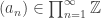 .
.
One might be tempted to think that all elements of can be realized as products of infinite sequences of shrinking loops like ![[\alpha]=g_1g_2g_3...](https://s0.wp.com/latex.php?latex=%5B%5Calpha%5D%3Dg_1g_2g_3...&bg=ffffff&fg=333333&s=0&c=20201002) but alas, this is also too much to hope for. Not only is this too much to hope for, but the combinatorial structure of is far from free [3] since we can have “infinite” cancellations of the letters
but alas, this is also too much to hope for. Not only is this too much to hope for, but the combinatorial structure of is far from free [3] since we can have “infinite” cancellations of the letters  when we multiply two elements. See this post for a proof of non-freeness. As a first example, notice that
 ![[\alpha]^{-1}](https://s0.wp.com/latex.php?latex=%5B%5Calpha%5D%5E%7B-1%7D&bg=ffffff&fg=333333&s=0&c=20201002) can be thought of as the infinite word
can be thought of as the infinite word  and the product
 ![g_1 g_2 g_3......g_{3}^{-1} g_{2}^{-1} g_{1}^{-1}=[\alpha][\alpha]^{-1}=e](https://s0.wp.com/latex.php?latex=g_1+g_2+g_3......g_%7B3%7D%5E%7B-1%7D+g_%7B2%7D%5E%7B-1%7D+g_%7B1%7D%5E%7B-1%7D%3D%5B%5Calpha%5D%5B%5Calpha%5D%5E%7B-1%7D%3De&bg=ffffff&fg=333333&s=0&c=20201002) is the identity element. In more geometric terms, this means we can construct a null-homotopy of
is the identity element. In more geometric terms, this means we can construct a null-homotopy of  by nesting “small null-homotopies” of the loops
  inside of each other.
You can take this one-step further by considering the following iterative construction. Start with

Now insert more trivial pairs, but make the index of the  ‘s get larger at each step so the construction is actually represented by a continuous loop.

 (cont. on next line)


At every stage and in the limit, this construction should represent the identity element of the group, however, in the “transfinite word” which is the limit, there are no straightforward cancellation pairs  to be found anywhere! This is because we went on to put new letters in the middle of every such pair. So the cancellations that go on in can be quite subtle. How could you possibly define a loop representing the above word? Well, if you look closely at where new pairs are inserted, you can see that it has a “Cantor set-ish” feel to it.
To describe loops representing all elements of  , we call upon the middle-third Cantor set
 ![{C}\subset {[0,1]}](https://s0.wp.com/latex.php?latex=%7BC%7D%5Csubset+%7B%5B0%2C1%5D%7D&bg=ffffff&fg=333333&s=0&c=20201002) . There are countably many open intervals
. There are countably many open intervals ![{[0,1]}{\backslash}{C}=\bigcup_{k\geq 1}(a_k,b_k)](https://s0.wp.com/latex.php?latex=%7B%5B0%2C1%5D%7D%7B%5Cbackslash%7D%7BC%7D%3D%5Cbigcup_%7Bk%5Cgeq+1%7D%28a_k%2Cb_k%29&bg=ffffff&fg=333333&s=0&c=20201002) . We can define a loop by defining
. We can define a loop by defining  and defining
  on
on ![[a_k,b_k]](https://s0.wp.com/latex.php?latex=%5Ba_k%2Cb_k%5D&bg=ffffff&fg=333333&s=0&c=20201002) to either be the constant loop or to be one of the loops
to either be the constant loop or to be one of the loops  for some
  . We have one restriction to ensure that is continuous. We must ensure that for each
  , we only have
  for finitely many
  . This means for fixed
  , the loops and can only be used finitely many times. Otherwise, we would admit infinite concatenations like
  which clearly cannot be continuous. It turns out that any element of
  is represented by a loop constructed in this way. You can convince yourself of this by first noticing that for any loop , the preimage
  is a countable union of disjoint open intervals.
We’ve yet to really compute . We could argue exactly what I mean by “compute” here but I really mean “identify the isomorphism class” as a reasonably familiar group so that we can make formal algebraic arguments about the group structure without appealing to loops. This is done using shape theory. Before we continue, I should mention that this shape theoretic approach can fail to provide an explicit characterization of  when you start considering subsets of
  .
.
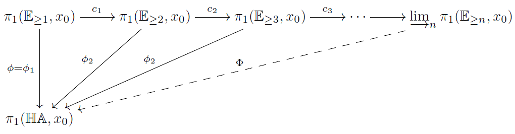
Recall that one way to construct is as an inverse limit where where  is the union of the first n-circles. Note that
  is the free group on the generators
  . If we apply the fundamental group
  to the entire inverse system
,
we get an inverse system of free groups

where the homomorphism  collapses
  to the identity. The inverse limit
  is the first shape group of . To be fair, the shape group cannot always be constructed in this way but this is a nice way to understand the one-dimensional case.
We also have projections  which collapse
  to the basepoint for
  . The induced homomorphisms
  clearly agree with the bonding homomorphisms
  in the inverse system of free groups so we get an induced homomorphism
  to the first shape group.
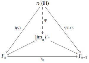
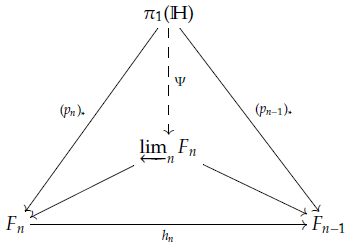
The inverse limit of free groups  is constructed as a subgroup of
  . Specifically, consists of the sequences
  of words
  such that
 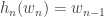 . This means we can think of elements of as sequences of words where the word
  (in letters
  ) is obtained from the word
  (in letters
  ) by removing all instances of the letter
  . The homomorphism
  is defied as
 ![\Psi([\alpha])=(w_n)](https://s0.wp.com/latex.php?latex=%5CPsi%28%5B%5Calpha%5D%29%3D%28w_n%29&bg=ffffff&fg=333333&s=0&c=20201002) where
where ![w_n=[p_n\circ\alpha]\in F_n](https://s0.wp.com/latex.php?latex=w_n%3D%5Bp_n%5Ccirc%5Calpha%5D%5Cin+F_n&bg=ffffff&fg=333333&s=0&c=20201002) .
.
The key to understanding is the following theorem which originally appeared in a paper of H.B. Griffiths [1]. Griffiths’ proof apparently had some sort of error in it; a corrected proof was given by Morgan and Morrison [2] and many have since appeared.
Shape Injectivity Theorem: is injective.
One way to prove this theorem is to use the data of infinite “word reduction” to construct a null-homotopy of a loop such that ![\Psi([\alpha])=1](https://s0.wp.com/latex.php?latex=%5CPsi%28%5B%5Calpha%5D%29%3D1&bg=ffffff&fg=333333&s=0&c=20201002) (equivalently
(equivalently ![[p_n\circ \alpha]=1\in \pi_1(X_n)=F_n](https://s0.wp.com/latex.php?latex=%5Bp_n%5Ccirc+%5Calpha%5D%3D1%5Cin+%5Cpi_1%28X_n%29%3DF_n&bg=ffffff&fg=333333&s=0&c=20201002) for each ). It is helpful to imagine doing this for the example above where we kept inserting trivial pairs
for each ). It is helpful to imagine doing this for the example above where we kept inserting trivial pairs  between trivial pairs and so on. The details of a full proof are somewhat non-trivial so I’ll skip it for now (but plan to come back to it later). The upshot of the theorem is that we can now understand elements of
  as sequences of words in
  .
.
The question then remains: what is the image of ?
Proposition: 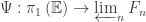 is not surjective.
Consider the sequence  of commutators
  . Note that as
  the number of appearances of
  grows without bound. But we can’t have a loop
 ![{\alpha} :{[0,1]}\to\mathbb{E}](https://s0.wp.com/latex.php?latex=%7B%5Calpha%7D+%3A%7B%5B0%2C1%5D%7D%5Cto%5Cmathbb%7BE%7D&bg=ffffff&fg=333333&s=0&c=20201002) that corresponds to this element since no continuous loop can traverse
that corresponds to this element since no continuous loop can traverse  infinitely many times. This geometric restriction suggests which subgroup we should be looking for.
Definition: If  and
and  , let
, let  be the number of times
  appears in the reduced word
  . We say an element is locally eventually constant if for each
  , the sequence
  is eventually constant (as
  ). Let
  be the subgroup of locally eventually constant sequences.
If ![\Psi ([\alpha])=(w_n)](https://s0.wp.com/latex.php?latex=%5CPsi+%28%5B%5Calpha%5D%29%3D%28w_n%29&bg=ffffff&fg=333333&s=0&c=20201002) is not locally eventually constant, then we’d have some
is not locally eventually constant, then we’d have some  where the number of times appears is unbounded and this contradicts the continuity of . On the other hand, our method of using the Cantor set to construct loops provides a nice way to represent every locally eventually constant sequence by a continuous loop. We conclude that the locally eventually constant sequences are precisely the sequences corresponding to continuous loops.
Theorem [2]:  embeds isomorphically onto
  .
.
The group  is sometimes called the free
  -product of
  in infinite group theory.
Summary
Let’s sum up this combinatorial description of : The fundamental group of the earring space is isomorphic to the group of sequences where
- is a reduced word in the free group on letters
 ,
,
- removing the letter from gives the word ,
- for each
 , the number of times the letter
  appears in stabilizes at (i.e. the sequence
  is eventually constant for each ).
References.
[1] H.B. Griffiths, Infinite products of semigroups and local connectivity, Proc. London Math. Soc. (3), 6 (1956), 455-485.
[2] J. Morgan, I. Morrison, A van kampen theorem for weak joins, Proc. London Math. Soc. 53 (1986) 562–576.
[3] B. de Smit, The fundamental group of the Hawaiian earring is not free, Internat. J. Algebra Comput. 2 (1) (1992) 33–37.
Another great reference on the earring group is
[4] J.W. Cannon, G.R. Conner, The combinatorial structure of the Hawaiian earring group, Topology Appl. 106 (2000) 225-271.


be the n-th circle so that
.
be the smaller copies of the earring space.
be the open disk between
which contains the n-th hill in the archipelago.
be the open disk which is the upper half of the hill
.


![[\ell_{n}]=[\ell_{n+1}]](https://s0.wp.com/latex.php?latex=%5B%5Cell_%7Bn%7D%5D%3D%5B%5Cell_%7Bn%2B1%7D%5D&bg=ffffff&fg=333333&s=0&c=20201002)


![\phi([\ell_m])=\phi([\ell_n])](https://s0.wp.com/latex.php?latex=%5Cphi%28%5B%5Cell_m%5D%29%3D%5Cphi%28%5B%5Cell_n%5D%29&bg=ffffff&fg=333333&s=0&c=20201002)

![g_n=[\ell_n]\in\pi_1(\mathbb{E},x_0)](https://s0.wp.com/latex.php?latex=g_n%3D%5B%5Cell_n%5D%5Cin%5Cpi_1%28%5Cmathbb%7BE%7D%2Cx_0%29&bg=ffffff&fg=333333&s=0&c=20201002)


![[\alpha]\in\pi_1(\mathbb{E},x_0)=\pi_1(\mathbb{E}_{\geq 1},x_0)](https://s0.wp.com/latex.php?latex=%5B%5Calpha%5D%5Cin%5Cpi_1%28%5Cmathbb%7BE%7D%2Cx_0%29%3D%5Cpi_1%28%5Cmathbb%7BE%7D_%7B%5Cgeq+1%7D%2Cx_0%29&bg=ffffff&fg=333333&s=0&c=20201002)
![\phi([\alpha])=1](https://s0.wp.com/latex.php?latex=%5Cphi%28%5B%5Calpha%5D%29%3D1&bg=ffffff&fg=333333&s=0&c=20201002)
![c_{n-1}\circ c_{n-2}\circ\dots\circ c_1([\alpha])=1](https://s0.wp.com/latex.php?latex=c_%7Bn-1%7D%5Ccirc+c_%7Bn-2%7D%5Ccirc%5Cdots%5Ccirc+c_1%28%5B%5Calpha%5D%29%3D1&bg=ffffff&fg=333333&s=0&c=20201002)

![H:[0,1]\times[0,1]\to\mathbb{HA}](https://s0.wp.com/latex.php?latex=H%3A%5B0%2C1%5D%5Ctimes%5B0%2C1%5D%5Cto%5Cmathbb%7BHA%7D&bg=ffffff&fg=333333&s=0&c=20201002)

![G:[0,1]\times[0,1]\to\mathbb{E}_{\geq n}](https://s0.wp.com/latex.php?latex=G%3A%5B0%2C1%5D%5Ctimes%5B0%2C1%5D%5Cto%5Cmathbb%7BE%7D_%7B%5Cgeq+n%7D&bg=ffffff&fg=333333&s=0&c=20201002)


![f(g_n)=[\beta_n]](https://s0.wp.com/latex.php?latex=f%28g_n%29%3D%5B%5Cbeta_n%5D&bg=ffffff&fg=333333&s=0&c=20201002)
![[\alpha]\in \pi_1(\mathbb{E},x_0)](https://s0.wp.com/latex.php?latex=%5B%5Calpha%5D%5Cin+%5Cpi_1%28%5Cmathbb%7BE%7D%2Cx_0%29&bg=ffffff&fg=333333&s=0&c=20201002)


![[\alpha]\in\pi_1(\mathbb{E},x_0)](https://s0.wp.com/latex.php?latex=%5B%5Calpha%5D%5Cin%5Cpi_1%28%5Cmathbb%7BE%7D%2Cx_0%29&bg=ffffff&fg=333333&s=0&c=20201002)
![[\alpha]\in \ker\phi](https://s0.wp.com/latex.php?latex=%5B%5Calpha%5D%5Cin+%5Cker%5Cphi&bg=ffffff&fg=333333&s=0&c=20201002)


![\{[\alpha_j]\mid j\in J\}](https://s0.wp.com/latex.php?latex=%5C%7B%5B%5Calpha_j%5D%5Cmid+j%5Cin+J%5C%7D&bg=ffffff&fg=333333&s=0&c=20201002)


 of circles and the one-dimensional space
 , which induces an isomorphism on all homotopy groups. However,
  of our space
  , the open cover still gives a vague picture of
  as a subspace of the plane.


 and a set
  consisting of finite subsets of
  and
and  , then
  . A vertex or 0-simplex is a singleton
  and an n-simplex is a set
  containing
  elements. The n-skeleton of
 called the nerve of
  such that
  . The geometric realization
  is a geometric complex obtained by pasting simplices together using
  is the topological space
  defined as a subset of the product
 ![P=[0,1]^{K_0}](https://s0.wp.com/latex.php?latex=P%3D%5B0%2C1%5D%5E%7BK_0%7D&bg=ffffff&fg=333333&s=0&c=20201002) of functions
of functions ![f:K_0\to [0,1]](https://s0.wp.com/latex.php?latex=f%3AK_0%5Cto+%5B0%2C1%5D&bg=ffffff&fg=333333&s=0&c=20201002) . In particular,
. In particular,  such that
 (in particular all but finitely many
  are zero),
 .
. the weak (or induced) topology so that
  is open in
 ![U\cap [0,1]^{F}](https://s0.wp.com/latex.php?latex=U%5Ccap+%5B0%2C1%5D%5E%7BF%7D&bg=ffffff&fg=333333&s=0&c=20201002) is open in
is open in ![[0,1]^{F}](https://s0.wp.com/latex.php?latex=%5B0%2C1%5D%5E%7BF%7D&bg=ffffff&fg=333333&s=0&c=20201002) for all finite sets
for all finite sets  .
.  in
in ![[s_1,...,s_n]=\{f\in |K||f(s_i)>0\text{ for some }1\leq i\leq n\}](https://s0.wp.com/latex.php?latex=%5Bs_1%2C...%2Cs_n%5D%3D%5C%7Bf%5Cin+%7CK%7C%7Cf%28s_i%29%3E0%5Ctext%7B+for+some+%7D1%5Cleq+i%5Cleq+n%5C%7D&bg=ffffff&fg=333333&s=0&c=20201002) .
.


 , then place an edge (1-simplex) between
  and
and  .
.
 , then there are three edges joining each pair of the vertices
  . Place a triangle (or 2-simplex) so that the edges of the triangle match up with these three edges. In the picture, fill in the each empty triangle with a triangle.
 , attach a tetrahedron to fill in the boundary that exists from the four triangles.
 lies in
  .
. .
. is a refinement of another cover
  there is a
  .
. is “larger” than
  . The map
  induced on geometric realizations is unique up to homotopy.
 on vertices (i.e. elements of
  for
for  , define
  . If
. If  , then clearly
  so we define
 ![[V,V']](https://s0.wp.com/latex.php?latex=%5BV%2CV%27%5D&bg=ffffff&fg=333333&s=0&c=20201002) spanned by
spanned by  and
and  to the 1-simplex
 ![\left[U_{V},U_{V'}\right]](https://s0.wp.com/latex.php?latex=%5Cleft%5BU_%7BV%7D%2CU_%7BV%27%7D%5Cright%5D&bg=ffffff&fg=333333&s=0&c=20201002) spanned by
spanned by  and
and  . Any map defined in this way is called a projection.
 , then
  and we send the simplex
 ![[V_1,\dots,V_n]](https://s0.wp.com/latex.php?latex=%5BV_1%2C%5Cdots%2CV_n%5D&bg=ffffff&fg=333333&s=0&c=20201002) to
to ![[U_{V_{1}},...,U_{V_{n}}]](https://s0.wp.com/latex.php?latex=%5BU_%7BV_%7B1%7D%7D%2C...%2CU_%7BV_%7Bn%7D%7D%5D&bg=ffffff&fg=333333&s=0&c=20201002) . This gives a well-defined simplicial map on the nerves.
. This gives a well-defined simplicial map on the nerves. induce contiguous maps on geometric realizations. But contiguous maps of simplicial complexes are homotopic, proving the proposition.
  is a refinement of
  is a canonical map. Thus if
  is another projection, then there is a homotopy
  . Now if we let
 ![[p_{\mathscr{V}\mathscr{U}}]](https://s0.wp.com/latex.php?latex=%5Bp_%7B%5Cmathscr%7BV%7D%5Cmathscr%7BU%7D%7D%5D&bg=ffffff&fg=333333&s=0&c=20201002) denote the homotopy class of
denote the homotopy class of  , we have strict equality
 ![[p_{\mathscr{W}\mathscr{U}}] = [p_{\mathscr{V}\mathscr{U}}] \circ [p_{\mathscr{W}\mathscr{V}}]](https://s0.wp.com/latex.php?latex=%5Bp_%7B%5Cmathscr%7BW%7D%5Cmathscr%7BU%7D%7D%5D+%3D+%5Bp_%7B%5Cmathscr%7BV%7D%5Cmathscr%7BU%7D%7D%5D+%5Ccirc+%5Bp_%7B%5Cmathscr%7BW%7D%5Cmathscr%7BV%7D%7D%5D&bg=ffffff&fg=333333&s=0&c=20201002) . Therefore, since open covers of
. Therefore, since open covers of  , we have an inverse system
 ![\left(|N(\mathscr{U})|,[p_{\mathscr{V}\mathscr{U}}],\mathcal{O}(X)\right)](https://s0.wp.com/latex.php?latex=%5Cleft%28%7CN%28%5Cmathscr%7BU%7D%29%7C%2C%5Bp_%7B%5Cmathscr%7BV%7D%5Cmathscr%7BU%7D%7D%5D%2C%5Cmathcal%7BO%7D%28X%29%5Cright%29&bg=ffffff&fg=333333&s=0&c=20201002) of homotopy classes of nerves of covers.
of homotopy classes of nerves of covers. .
.