This is a guest post by Patrick Gillespie, who is currently a 2nd year Ph.D. student at the University of Tennessee Knoxville.

The Hopf map is a classical example of a non-trivial fiber bundle. There are many great visualizations of the Hopf map which depict the fibers of various points in . For example, Niles Johnson has a particularly good video which does this. These visualizations give a great deal of insight into the structure of the Hopf map, but I still felt as though I couldn’t see the Hopf map. So in this blog post, we will take an alternative approach to visualizing the Hopf map where we regard it as a loop of maps from the 2-sphere to itself. The identity map , whose homotopy class generates can be viewed as a loop of maps and the result can be animated as shown below. We will do the same with the Hopf map viewed as a loop of maps . We’ll also take a look at another map, which is homotopic to the Hopf map, but visually simpler to understand. The post will conclude with a discussion of the -homomorphism and how it can be used to visualize maps representing generators of for .

First, let and denote the reduced suspension and loop space of a pointed space , let be the space of pointed maps between two pointed spaces and , and let be the space of maps of pairs . By the loop-space suspension adjunction, recall that and are naturally homeomorphic, and this homeomorphism induces an isomorphism of groups of pointed homotopy classes . Since , we have that

Thus we may identify any map with a loop in , or equivalently, a loop in where is the closed unit disk, .

To express the Hopf map this way, we will first identify the Hopf map with a map . So let and find a homeomorphism between the interior of and . By identifying with , we may extend to a map . If denotes the Hopf map, let . We may identify and via the homeomorphism

induced by . Now for , let denote the restriction of to the disk . Then for each , and defines a loop .

Below is the animation of the Hopf map represented this way. At time , the left animation simply shows the domain of , regarded as a subspace of . The right animation shows the image of at time . The basepoint of is .

It is a bit hard to keep track of what is going on in this animation since the maps are not injective. To partially fix this, we can instead find a loop of maps which, after composing with the projection , is homotopic to . Very briefly, if , the idea will be to map circles of the form in via the Hopf map to a sphere with radius and centered at , where is a continuous function of both and satisfying a couple key properties. Importantly, if or if , then we want in order to guarantee that all of the maps share a consistent basepoint: in this case. The resulting loop of maps is animated below. We also include a point at the origin in the animation for reference.

This animation makes it a little easier to see how the Hopf map “loops” around the sphere. In particular, notice that the blue potion does twist around completely but that the red arcs only trace out disks. To simplify things even further, consider the following animation where both the red and blue arcs are “straightened out.”

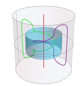
Let be the map represented by the above animation. An explicit homotopy between and was a by-product of constructing and can be found here. The description of the homotopy is tedious so I’ll leave it in the attached pdf. For some intuition as to why the two maps should be homotopic, one can check that, for , the fibers of a general pair of points form linked topological circles. The fibers of , , , and are shown below in red, blue, green, and purple respectively ( is not included in the picture of the fiber of ).

Note that while the fiber of is not a circle, it is a cylinder and thus homotopic to a circle. Also, while the fiber of is the union of the with red line shown, the image of this fiber under the identification is homeomorphic to a circle.

Before we continue, let’s quickly establish some notation that will help us break down, not just loops, but some paths in . For paths such that , let denote the concatenation of and . Let denote the reverse of , i.e. . Finally, if is a loop, let be the -fold concatenation of with itself, where , and let be the constant loop at .

Viewing as a map , we may write where and are simply restricted to time intervals and respectively. Because can be represented as a genuine path-conjugate, it follows that the -th power of is . If we were to animate , we would see the blue sphere rotate times (clockwise or counterclockwise depending on the sign of .) The takeaway here is that we have a visual correspondence between loops of rotations which fix a point, which we can think of as representatives of elements of , and powers of the Hopf map. We are seeing the -homomorphism in action!

The -homomorphism is really a collection of homomorphisms originally defined by Whitehead as follows. An element of restricts to an unbased map and this defines a map . Then given representing an element of , the composition is equivalent to a map by the exponential law. Applying the Hopf construction to this, we obtain a map . Since and , we define by setting .

However, there is a equivalent definition of the -homomorphism which will be more useful for our purposes. Consider the map in which an element of is sent to a based map by taking one-point compactifications (and where the basepoint is ). Then we can equivalently define the -homomorphism as the map induced by .

We glossed over some subtleties in the second definition. If we wish to work on the level of representatives, a map is sent to for which the basepoint of is sent to the identity map in rather than the constant map. Hence we cannot immediately apply the loop-space suspension adjunction to obtain a map as we might wish. Instead we should compose with a homotopy equivalence which sends the path component of the identity map to the path component of the constant map (for example, we could take to be the homotopy equivalence induced by multiplying by an element of of degree ). Then given , the composition maps to the path component of the constant map. Finally, through a change of basepoints, we obtain in which the basepoint of is sent to the constant map. We can then identify this with a map which represents the image of under the -homomorphism.

I’d like to draw our attention back to the map , where as before, and are restricted to and respectively. At each time , the regions shaded red and blue in the animation of correspond to the northern and southern hemispheres of in the domain of , which we will denote and respectively. Now define by setting , that is, we restrict to the blue hemisphere at each time . Strictly speaking, is a map , but this is of course equivalent to a map . Then from the animation of , we see that factors as the composition where represents a generator of and is the map used in the definition of the -homomorphism. Note that extending to amounts to composing with a homotopy equivalence which maps the path component of the identity map to that of the constant map. Finally, is the result of conjugating by the path . Not only does this show that is the image of a generator of under the -homomorphism, but it also shows how we could have arrived at the visualization of through our second definition of the -homomorphism.

With this in mind, we will now attempt to visualize the images of the homomorphisms for all . It is classical that the -homomorphism is an isomorphism in these cases, hence this will allow us to visually understand generators of for all . In order to do this, we first present an alternative way of visualizing the map which will be much easier to generalize. At each time , we may identify the domain of with the union of and glued together along their boundaries in the obvious way. We may also regard the codomain of as the quotient of in which the boundary is collapsed to a single point. Then we may visualize as shown below through two side-by-side animations where, at time , the left animation shows the image of restricted to the northern hemisphere , and the right animation shows the image of restricted to the southern hemisphere . In the animation, the dotted circle represents the boundary which we regard as a single point in .

What you’re seeing here is simply an alternative way to visualize the previous animation (of ). Technically, the above animation depicts a map , homotopic to , but for which the conjugating path differs from very slightly. You have to look pretty closely to observe the difference between and . As time progresses, both and pull the equator up toward the north pole. However, the way in which does this is not perfectly symmetric – at the start and end of the animation you can see a little more red than blue – whereas the expansion and shrinking of disks in this animation using is symmetric. This difference is certainly not homotopically significant.

We can now generalize this visualization to loops representing generators of for all . For example, below is an animation in the same style as above, but now representing a map . If and are two hemispheres of (each of which is homeomorphic to a closed -ball,) at each time , the image of restricted to and is shown on the left and right respectively.

Analogous to how we saw that was the image of a generator under the -homomorphism, one can similarly check that the is the image of a generator under the -homomorphism. Hence indeed generates .

Although we cannot animate the loops for as we have run out of spatial dimensions to work with, there is a clear pattern, which provides at least some visual understanding of the elements of .