
In Infinite Commutativity: Part I, I described infinite commutativity in general terms with some basic examples, including real infinite series. In this post, I’ll discuss how the homotopy groups 


History and Recent Work
The idea that higher homotopy groups are infinitely commutative is only 20 years old (due to Eda-Kawamura) because the proof is fairly intricate and it could easily seem overwhelming if you don’t already know how it goes. You can find it implicitly built into the main proof in [3] but even though I understand the fundamental ideas of the proof, beware that the details there are difficult to read. This idea was also used by Kawamura in [4] to study the higher dimensional earrings (sometimes called Barratt-Milnor Spheres) Following [3] and [4], infinite commutativity in 
In the effort to formalize the infinite product framework for pushing the homotopy theory of locally complicated spaces, I’ve worked both on infinite commutativity in fundamental groups with a former student [2] and also higher homotopy groups in [1]. Part of my recent work in [1] and [2] is to make this business all more practical for computations and future applications. So I’ve been trying to formalize, simplify, and strengthen the set of available tools. This kind of math is really fun (in my opinion) and has potential to open up a lot of new avenues for research. The truth is that, right now, there are many fundamental and important open questions related to wild higher homotopy groups that are likely to become more accessible with the development of new tools/foundations, so lately I’ve been thinking a lot about these ideas.
Infinite Products in Higher Homotopy Groups
Let’s start with ordinary infinite products indexed by the natural numbers at the n-th loop space level. Since we’re talking about higher homotopy, 
For a based space 


Definition: Let 


If 


Let’s start with the obvious first choice: given a null-sequence of maps 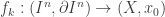

![\left[1-\frac{1}{2^{k-1}},1-\frac{1}{2^{k}}\right]\times I^{n-1}](https://s0.wp.com/latex.php?latex=%5Cleft%5B1-%5Cfrac%7B1%7D%7B2%5E%7Bk-1%7D%7D%2C1-%5Cfrac%7B1%7D%7B2%5E%7Bk%7D%7D%5Cright%5D%5Ctimes+I%5E%7Bn-1%7D&bg=ffffff&fg=333333&s=0&c=20201002)


Infinite product of 2-loops
By taking the homotopy class of 
![\{f_k\}_{k=1}^{\infty}\mapsto\left[\prod_{k=1}^{\infty}f_k\right]](https://s0.wp.com/latex.php?latex=%5C%7Bf_k%5C%7D_%7Bk%3D1%7D%5E%7B%5Cinfty%7D%5Cmapsto%5Cleft%5B%5Cprod_%7Bk%3D1%7D%5E%7B%5Cinfty%7Df_k%5Cright%5D&bg=ffffff&fg=333333&s=0&c=20201002)

Warning/Red Alert!! We may want to jump quickly to writing down a partially-defined infinite sum operation of homotopy classes by setting ![\sum_{k=1}^{\infty}[f_k]=\left[\prod_{k=1}^{\infty}f_k\right]](https://s0.wp.com/latex.php?latex=%5Csum_%7Bk%3D1%7D%5E%7B%5Cinfty%7D%5Bf_k%5D%3D%5Cleft%5B%5Cprod_%7Bk%3D1%7D%5E%7B%5Cinfty%7Df_k%5Cright%5D&bg=ffffff&fg=333333&s=0&c=20201002)
![\{[f_k]\}_{k=1}^{\infty}\mapsto\left[\prod_{k=1}^{\infty}f_k\right]](https://s0.wp.com/latex.php?latex=%5C%7B%5Bf_k%5D%5C%7D_%7Bk%3D1%7D%5E%7B%5Cinfty%7D%5Cmapsto%5Cleft%5B%5Cprod_%7Bk%3D1%7D%5E%7B%5Cinfty%7Df_k%5Cright%5D&bg=ffffff&fg=333333&s=0&c=20201002)


Here’s how infinite commutativity works for these particular kinds of infinite products:
Lemma: If 


Idea of the Proof. Let’s not do a technical proof here. Instead, let’s just see how this is done in pictures in dimension 


is homotopic to


Our pictures will look a lot like the Eckmann-Hilton gif from Part I but with infinitely many rectangles sliding around instead of just two. I’m afraid that I wasn’t ambitious enough to animate this so all you’ll get is a sequence of still images.
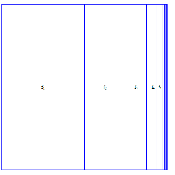
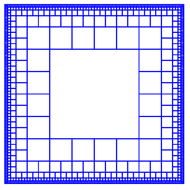
Throughout the following sequence of steps, the blue squares will represent the domain of the maps 


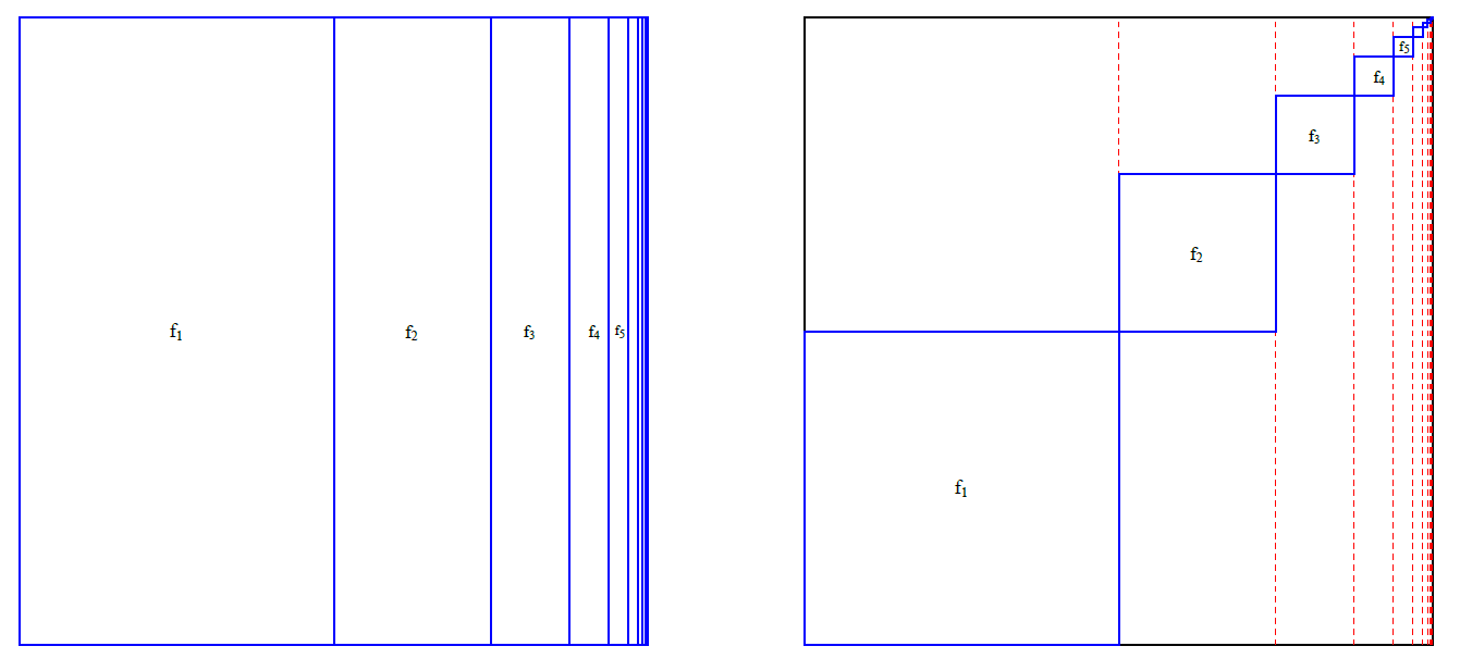
Now that we’ve done a vertical “reparameterization” we want to switch to a horizontal slide/stretch. This is where 


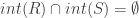
Now that we’ve taken care of things horizontally, it’s now a matter of some more vertical stretching to ensure that what we end up with is precisely an infinite product.

Finally, we end up with 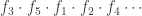

![H:[0,1]^3\to X](https://s0.wp.com/latex.php?latex=H%3A%5B0%2C1%5D%5E3%5Cto+X&bg=ffffff&fg=333333&s=0&c=20201002)

Eckmann Hilton Homotopy
Now imagine the same animation in this situation. There will be infinitely many cylinders ![S_1,S_2,S_3,...\subseteq [0,1]^3](https://s0.wp.com/latex.php?latex=S_1%2CS_2%2CS_3%2C...%5Csubseteq+%5B0%2C1%5D%5E3&bg=ffffff&fg=333333&s=0&c=20201002)
![[0,1]^3](https://s0.wp.com/latex.php?latex=%5B0%2C1%5D%5E3&bg=ffffff&fg=333333&s=0&c=20201002)


![[0,1]^3\backslash \bigcup_{k=1}^{\infty}int(S_k)](https://s0.wp.com/latex.php?latex=%5B0%2C1%5D%5E3%5Cbackslash+%5Cbigcup_%7Bk%3D1%7D%5E%7B%5Cinfty%7Dint%28S_k%29&bg=ffffff&fg=333333&s=0&c=20201002)


Hooray! We conclude that homotopy classes of infinite products in higher homotopy groups don’t change if you start shuffling around factors. So when infinite sums are well defined and the notation ![\sum_{k=1}^{\infty}[f_k]](https://s0.wp.com/latex.php?latex=%5Csum_%7Bk%3D1%7D%5E%7B%5Cinfty%7D%5Bf_k%5D&bg=ffffff&fg=333333&s=0&c=20201002)


Now you can imagine how this type of argument might be generalized and altered.
Definition: An n-domain is a (possibly infinite) collection 
![\prod_{m=1}^{n}[a_m,b_m]](https://s0.wp.com/latex.php?latex=%5Cprod_%7Bm%3D1%7D%5E%7Bn%7D%5Ba_m%2Cb_m%5D&bg=ffffff&fg=333333&s=0&c=20201002)
![[0,1]^n](https://s0.wp.com/latex.php?latex=%5B0%2C1%5D%5En&bg=ffffff&fg=333333&s=0&c=20201002)

The next step is to generalize the idea of infinite product to make sense for a general n-domain.
Definition: If 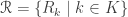


![[0,1]^n\backslash \bigcup_{k\in K}int(R_k)](https://s0.wp.com/latex.php?latex=%5B0%2C1%5D%5En%5Cbackslash+%5Cbigcup_%7Bk%5Cin+K%7Dint%28R_k%29&bg=ffffff&fg=333333&s=0&c=20201002)
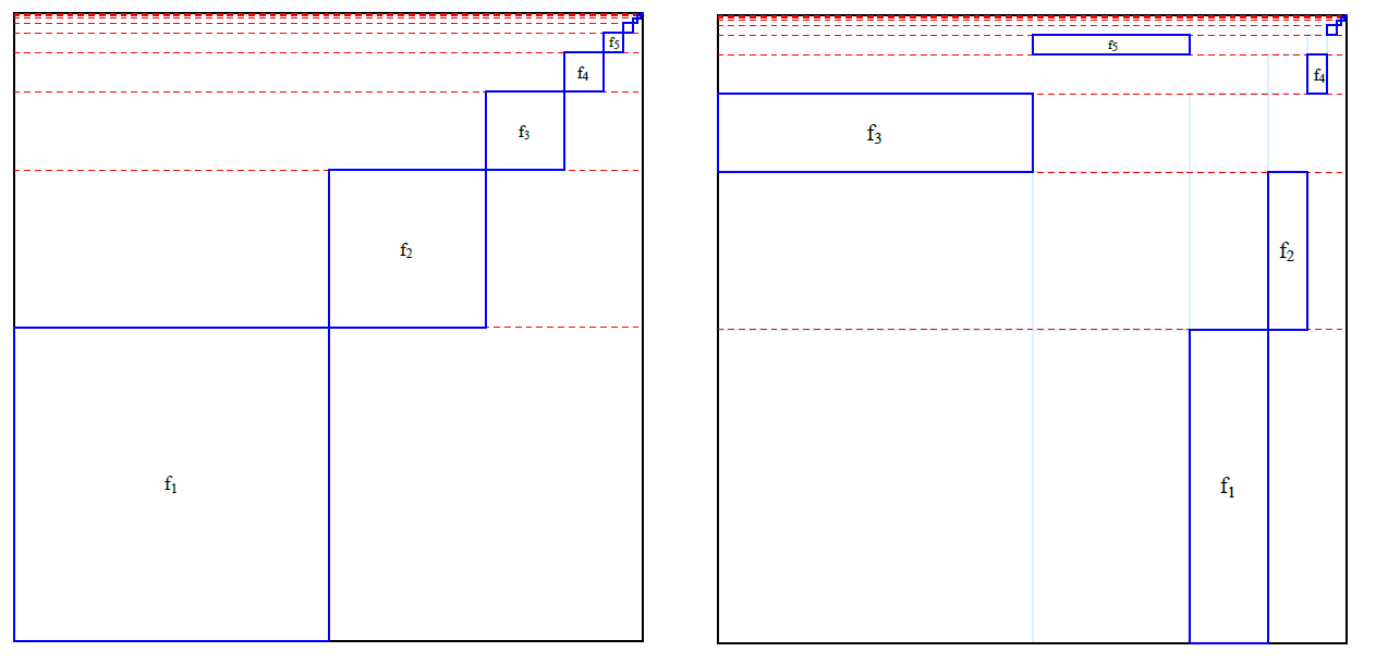
Be warned that n-domains are arbitrary.
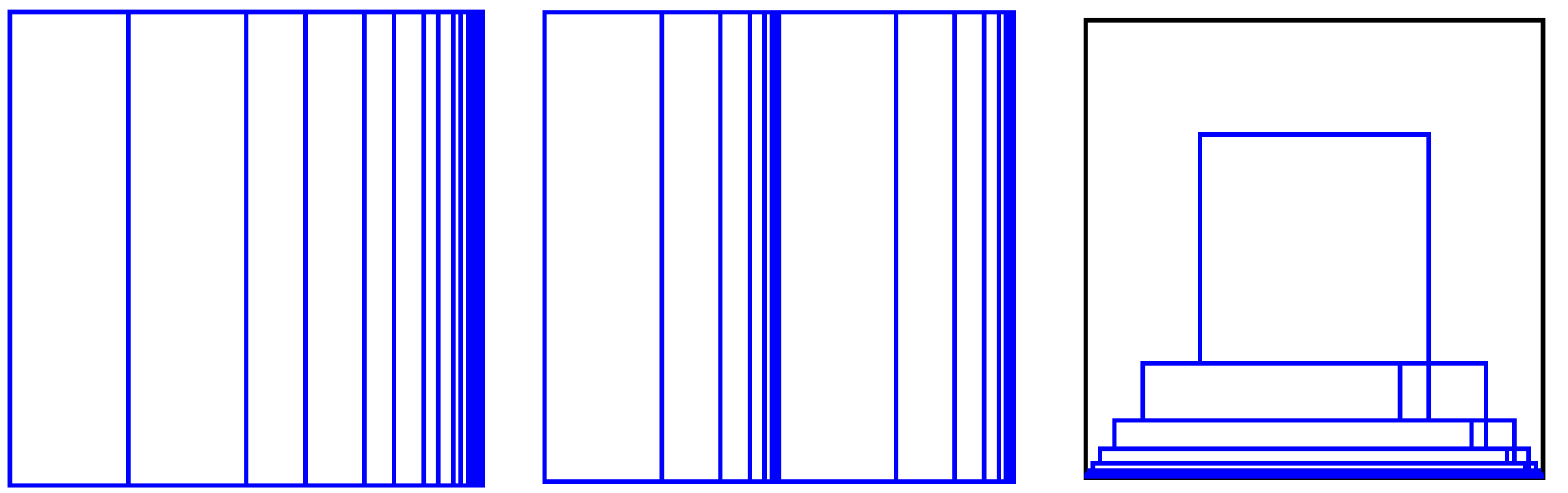
Some examples of 2-domains. Each rectangular region with a blue boundary is an element of the intended n-domain.
So the main question now is….
Question: Given any two n-domains 


I can’t help but spoiling it… The answer is YES! This is a Theorem in [1]. Here’s why you should be even more startled that the answer is YES…The approach we took (in the lemma) for simultaneously sliding around individual squares/cubes fails miserably in general. It fails when you run into an n-domain that look like this:
Yikes! There’s no way to make individual moves and hope to shuffle them (after some choice of ordering) back into the simple n-domain for infinite products. If you try to move individual squares (all at once or even finitely many at a time), you will end up breaking continuity. Remember our original n-domain for defining ordinary infinite products (on the right)? How do you continuously shuffle the squares in the complicated one above to align with these ones, all of which have height 1? Aren’t we turning arbitrarily small things into big things???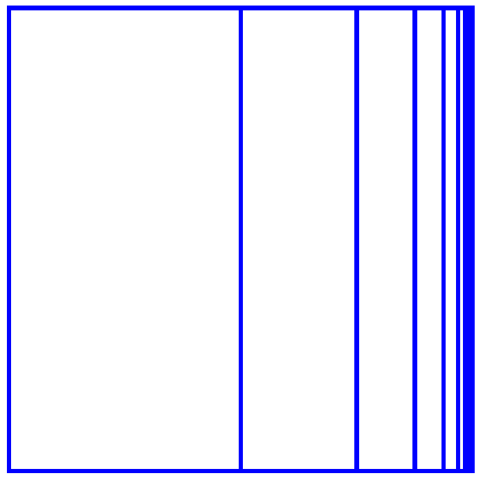
It seems like there’s just too much in the way and like sequences of squares that converge to the boundary are going to be a problem. Despite all this potential concern, there is a way to do it. Once you realize the main tricks, you have a ton of freedom to move things around in the domain while still holding a continuous homotopy in your hand at the end of the day. When I was writing the paper [1], I worked really hard to find the simplest geometric procedure I could possibly imagine to get the job done. The whole time, I was imagining these infinite swarms of rectangular cylinders twisting around each other in time just like the above gif with two cylinders. I had a lot of fun working it out and I am excited to see how this formalized interpretation of “infinite commutativity” will be applied.
So… not only are higher homotopy groups commutative for infinite products, they are commutative in this super-duper-geometric-infinite way.
A comment for operad fans
One cool thing here is the extension of the little 
For us infinitary-minded folks, we can take 
Just as 
References:
[1] J. Brazas, The infinitary n-cube shuffle. Topology Appl. 287 (2020) 107446. arXiv:2006.08738
[2] J. Brazas, P. Gillespie, Infinitary commutativity and abelianization in fundamental groups. (2020). To appear in the Journal of the Australian Math. Society.
[3] K. Eda, K. Kawamura, Homotopy and Homology Groups of the n-dimensional Hawaiian earring, Fund. Math. 165 (2000) 17-28.
[4] K. Kawamura, Low dimensional homotopy groups of suspensions of the Hawaiian earring, Colloq. Math. 96 (2003) no. 1 27-39.
 with two unital operations
  and
and  satisfying the distributive rule:
  . Using only this set-up, we have the following theorem.
 and
and  be the identity elements for the operations
  and
and  respectively. We check the desired equalities in sequence. Each argument uses a previous one.


 .
.  , we can define the concatenation n-loop
  by the formula:
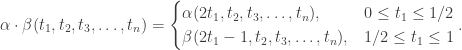
![[\alpha]+[\beta]:=[\alpha\cdot\beta]](https://s0.wp.com/latex.php?latex=%5B%5Calpha%5D%2B%5B%5Cbeta%5D%3A%3D%5B%5Calpha%5Ccdot%5Cbeta%5D&bg=ffffff&fg=333333&s=0&c=20201002) defines the group operation of
defines the group operation of ![[\alpha]+[\beta]=[\beta]+[\alpha]](https://s0.wp.com/latex.php?latex=%5B%5Calpha%5D%2B%5B%5Cbeta%5D%3D%5B%5Cbeta%5D%2B%5B%5Calpha%5D&bg=ffffff&fg=333333&s=0&c=20201002) . The following gif is basically a topological picture of the Eckmann-Hilton principle applied in dimension
. The following gif is basically a topological picture of the Eckmann-Hilton principle applied in dimension  . The blue rectangle is the domain of
  and the red rectangle is the domain of
  (with suitable scaling applied). The animation basically tells us how to define a homotopy from
  to
to  as a map on a solid cube by showing how to define it on each vertical slice. Think of the start (height
  ) as mapping the bottom of a cube
  on higher slices
 ![[0,1]^2\times\{t\}](https://s0.wp.com/latex.php?latex=%5B0%2C1%5D%5E2%5Ctimes%5C%7Bt%5C%7D&bg=ffffff&fg=333333&s=0&c=20201002) . Finally, the end (
. Finally, the end ( ) is how we map the top of the cube as
 ![H:[0,1]^2\times [0,1]\to X](https://s0.wp.com/latex.php?latex=H%3A%5B0%2C1%5D%5E2%5Ctimes+%5B0%2C1%5D%5Cto+X&bg=ffffff&fg=333333&s=0&c=20201002) from
from ![[\alpha]+[\beta]=[\alpha\cdot\beta]=[\beta\cdot\alpha]=[\beta]+[\alpha]](https://s0.wp.com/latex.php?latex=%5B%5Calpha%5D%2B%5B%5Cbeta%5D%3D%5B%5Calpha%5Ccdot%5Cbeta%5D%3D%5B%5Cbeta%5Ccdot%5Calpha%5D%3D%5B%5Cbeta%5D%2B%5B%5Calpha%5D&bg=ffffff&fg=333333&s=0&c=20201002) .
. has image in
  and, in fact, has constant image for all “time” of the homotopy. In particular, you can commute small loops with small homotopies.
 , which assigns an output (represented here using product notation) to certain infinite sequences in
  . For example if
  is another indexing set (typically with an ordering or some other structure on it), then an infinitary
  .
. . Chances are that if you’re reading this blog, you’ve seen these before.
 and
and  which have applications to fixed point theory and number theory. There are analogous infinitary sum/product operations for matrices.
 is a directed system in a category and
  is very much the infinite composition
  where
where  are the bonding maps. More generally, the canonical map
  is the infinite composition
  . The dual situation works for inverse limits and you can replace the naturals
  with any well-ordered indexing set. Sometimes this kind of thing is called transfinite composition. The unavoidable topology that creeps in is hiding in the fact that the ordered set
  of objects (including the colimit) is indexed by a non-discrete compact ordered set, namely
  . It is not a coincidence that
  .
. and demand that
  always holds.
 of the indexing set on the
  is invariant under the infinitary operation
  shrink to
  to ensure that
  is well-defined, e.g.
  diverges. Which sequences have a well-defined sum has more to do with the existence of a shrinking sequence of tails
  as I described for
 converges and there is a Rearrangement Theorem stating that if
  . A series is conditionally convergent if it is not absolutely convergent and the Rearrangement Theorem states that if
  is any real number, then there exists a bijection
  . For instance, the alternating harmonic series
  is conditionally convergent and its terms can be rearranged so the new sum converges to
  or
or  or whatever number you want.
 is the infinite direct product of discrete groups
  and consists of all infinite sequences of integers
  . We give
  of sequences converges to
  if and only if there initial coordinates in the sequence
  stabilize to the terms of
  , that is if for every
  , there exists an
  such that
  for all
  . So if you keep going through the sequence
  that converges to the identity, we can define a sum
  as the sequence
 is eventually
 , which means that the natural infinite sum operation on the Specker group is infinitely commutative. So, in an infinitary algebra sense, the Specker group is much simpler that the infinite series operation on the real line.
 of a fundamental group
  to “detect” when a covering map
  exists that corresponds to a given subgroup
  . In particular,
 denotes the reverse path of
 ![[\alpha][\beta]=[\alpha\cdot\beta]](https://s0.wp.com/latex.php?latex=%5B%5Calpha%5D%5B%5Cbeta%5D%3D%5B%5Calpha%5Ccdot%5Cbeta%5D&bg=ffffff&fg=333333&s=0&c=20201002) for the operation on path-homotopy classes.
for the operation on path-homotopy classes. be an open cover of a space
  where
where  for some
  . In short, it’s
![\pi(\mathscr{U},x_0)=\langle [\alpha\cdot\gamma\cdot\alpha^{-}]\in \pi_1(X,x_0)\mid \exists U\in\mathscr{U}\,\,Im(\gamma)\subseteq U\rangle](https://s0.wp.com/latex.php?latex=%5Cpi%28%5Cmathscr%7BU%7D%2Cx_0%29%3D%5Clangle+%5B%5Calpha%5Ccdot%5Cgamma%5Ccdot%5Calpha%5E%7B-%7D%5D%5Cin+%5Cpi_1%28X%2Cx_0%29%5Cmid+%5Cexists+U%5Cin%5Cmathscr%7BU%7D%5C%2C%5C%2CIm%28%5Cgamma%29%5Csubseteq+U%5Crangle&bg=ffffff&fg=333333&s=0&c=20201002)

![\prod_{i=1}^{n}[\alpha_i][\gamma_i][\alpha_{i}^{-}]](https://s0.wp.com/latex.php?latex=%5Cprod_%7Bi%3D1%7D%5E%7Bn%7D%5B%5Calpha_i%5D%5B%5Cgamma_i%5D%5B%5Calpha_%7Bi%7D%5E%7B-%7D%5D&bg=ffffff&fg=333333&s=0&c=20201002) where
where ![\alpha_i:([0,1],0)\to (X,x_0)](https://s0.wp.com/latex.php?latex=%5Calpha_i%3A%28%5B0%2C1%5D%2C0%29%5Cto+%28X%2Cx_0%29&bg=ffffff&fg=333333&s=0&c=20201002) are paths and each
are paths and each  is a loop with image in some member of
 ![[\beta][\alpha][\gamma][\alpha^{-}][\beta]^{-}=[\beta\cdot\alpha][\gamma][(\beta\cdot\alpha)^{-}]](https://s0.wp.com/latex.php?latex=%5B%5Cbeta%5D%5B%5Calpha%5D%5B%5Cgamma%5D%5B%5Calpha%5E%7B-%7D%5D%5B%5Cbeta%5D%5E%7B-%7D%3D%5B%5Cbeta%5Ccdot%5Calpha%5D%5B%5Cgamma%5D%5B%28%5Cbeta%5Ccdot%5Calpha%29%5E%7B-%7D%5D&bg=ffffff&fg=333333&s=0&c=20201002) of a generator
of a generator ![[\alpha][\gamma][\alpha^{-}]](https://s0.wp.com/latex.php?latex=%5B%5Calpha%5D%5B%5Cgamma%5D%5B%5Calpha%5E%7B-%7D%5D&bg=ffffff&fg=333333&s=0&c=20201002) still has the form of a generator of
still has the form of a generator of  is another point and
 ![\beta:[0,1]\to X](https://s0.wp.com/latex.php?latex=%5Cbeta%3A%5B0%2C1%5D%5Cto+X&bg=ffffff&fg=333333&s=0&c=20201002) is a path from
is a path from  to
to  ,
, ![\varphi_{\beta}([\eta])=[\beta\cdot\eta\cdot\beta^{-}]](https://s0.wp.com/latex.php?latex=%5Cvarphi_%7B%5Cbeta%7D%28%5B%5Ceta%5D%29%3D%5B%5Cbeta%5Ccdot%5Ceta%5Ccdot%5Cbeta%5E%7B-%7D%5D&bg=ffffff&fg=333333&s=0&c=20201002) is the basepoint-change isomorphism, then
is the basepoint-change isomorphism, then  .
. refines
  is contained in some
 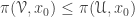 .
. : The cosets of Spanier groups form a basis for a topology on
  is open if for every
  , there exists an open cover
  . There are many topologies one can put on
  is a continuous function, then
  is an open cover of
  such that the induced homomorphism
  satisfies
  . I use the term continuity here because this is equivalent to saying that the induced homomorphisms
  are continuous with respect to the Spanier topology. Hence, the Spanier topology gives us one example of a fundamental group functor
  to the category of topological groups.
 be a 2-simplex with basepoint vertex
  and
and  be the 1-skeleton of some barycentric subdivision of
  be a map such that for every 2-simplex
  of
of  , we have
  for some
  of the outermost triangle factors as a huge product of “lasso” loops where the hoops of the lasso are the boundaries of the 2-simplices in the subdivision
  factors as a huge product of Spanier group generators and therefore represents an element
  if there exists an open neighborhood
  is trivial.
 , the induced homomorphism
  is trivial.
 since the covering space
  is inejctive) but this is a nice exercise to work out on it’s own.
  .
. be an open neighborhood of
  such that for every
  , the inclusion induces the trivial homomorphism
  , i.e. every loop in
  is an open cover of
 ![[\alpha\cdot\gamma\cdot\alpha^{-}]](https://s0.wp.com/latex.php?latex=%5B%5Calpha%5Ccdot%5Cgamma%5Ccdot%5Calpha%5E%7B-%7D%5D&bg=ffffff&fg=333333&s=0&c=20201002) of
of  has image in some
 ![\beta:[0,1]\to U_x](https://s0.wp.com/latex.php?latex=%5Cbeta%3A%5B0%2C1%5D%5Cto+U_x&bg=ffffff&fg=333333&s=0&c=20201002) from
from  . Now
. Now ![[\alpha\cdot\gamma\cdot\alpha^{-}]=[\alpha\cdot\beta][\beta\cdot\gamma\cdot\beta^{-}][\alpha\cdot\beta]^{-1}](https://s0.wp.com/latex.php?latex=%5B%5Calpha%5Ccdot%5Cgamma%5Ccdot%5Calpha%5E%7B-%7D%5D%3D%5B%5Calpha%5Ccdot%5Cbeta%5D%5B%5Cbeta%5Ccdot%5Cgamma%5Ccdot%5Cbeta%5E%7B-%7D%5D%5B%5Calpha%5Ccdot%5Cbeta%5D%5E%7B-1%7D&bg=ffffff&fg=333333&s=0&c=20201002) where
where  is a loop based a
 ![[\alpha\cdot\gamma\cdot\alpha^{-}]=[\alpha\cdot\beta][\beta\cdot\gamma\cdot\beta^{-}][\alpha\cdot\beta]^{-1}=[\alpha\cdot\beta][\alpha\cdot\beta]^{-1}=1](https://s0.wp.com/latex.php?latex=%5B%5Calpha%5Ccdot%5Cgamma%5Ccdot%5Calpha%5E%7B-%7D%5D%3D%5B%5Calpha%5Ccdot%5Cbeta%5D%5B%5Cbeta%5Ccdot%5Cgamma%5Ccdot%5Cbeta%5E%7B-%7D%5D%5B%5Calpha%5Ccdot%5Cbeta%5D%5E%7B-1%7D%3D%5B%5Calpha%5Ccdot%5Cbeta%5D%5B%5Calpha%5Ccdot%5Cbeta%5D%5E%7B-1%7D%3D1&bg=ffffff&fg=333333&s=0&c=20201002) . Since all the generators of
. Since all the generators of  be a path-connected neighborhood of
  for some
  refines
  . We check that the inclusion
  induces the trivial homomorphism on fundamental groups. If
 ![\gamma:([0,1],\{0,1\})\to (V_x,x)](https://s0.wp.com/latex.php?latex=%5Cgamma%3A%28%5B0%2C1%5D%2C%5C%7B0%2C1%5C%7D%29%5Cto+%28V_x%2Cx%29&bg=ffffff&fg=333333&s=0&c=20201002) is a loop, consider any path
is a loop, consider any path ![\alpha:[0,1]\to X](https://s0.wp.com/latex.php?latex=%5Calpha%3A%5B0%2C1%5D%5Cto+X&bg=ffffff&fg=333333&s=0&c=20201002) from
from ![[\alpha\cdot\gamma\cdot\alpha]](https://s0.wp.com/latex.php?latex=%5B%5Calpha%5Ccdot%5Cgamma%5Ccdot%5Calpha%5D&bg=ffffff&fg=333333&s=0&c=20201002) is generator of
is generator of  and must therefore, represent the identity element in
 ![[\alpha\cdot\gamma\cdot\alpha]=1](https://s0.wp.com/latex.php?latex=%5B%5Calpha%5Ccdot%5Cgamma%5Ccdot%5Calpha%5D%3D1&bg=ffffff&fg=333333&s=0&c=20201002) in
in ![[\gamma]=1](https://s0.wp.com/latex.php?latex=%5B%5Cgamma%5D%3D1&bg=ffffff&fg=333333&s=0&c=20201002) in
in  . Thus
  .
. , we have
  .
. . Let
. Let  and
and  be the end point of the lift
 ![\widetilde{\alpha}:([0,1],0\to (Y,y_0)](https://s0.wp.com/latex.php?latex=%5Cwidetilde%7B%5Calpha%7D%3A%28%5B0%2C1%5D%2C0%5Cto+%28Y%2Cy_0%29&bg=ffffff&fg=333333&s=0&c=20201002) of
of  containing
  that is mapped homeomorphically onto
  of
of  is a loop in
  . We have
 ![[\alpha\cdot\gamma\cdot\alpha^{-}]=p_{\#}([\widetilde{\alpha}\cdot\widetilde{\gamma}\cdot \widetilde{\alpha}^{-}])\in p_{\#}(\pi_1(Y,y_0))](https://s0.wp.com/latex.php?latex=%5B%5Calpha%5Ccdot%5Cgamma%5Ccdot%5Calpha%5E%7B-%7D%5D%3Dp_%7B%5C%23%7D%28%5B%5Cwidetilde%7B%5Calpha%7D%5Ccdot%5Cwidetilde%7B%5Cgamma%7D%5Ccdot+%5Cwidetilde%7B%5Calpha%7D%5E%7B-%7D%5D%29%5Cin+p_%7B%5C%23%7D%28%5Cpi_1%28Y%2Cy_0%29%29&bg=ffffff&fg=333333&s=0&c=20201002) . Since
. Since  contains all generators of
  such that
  if and only if there exists an open covering
  .
. be the set of “groupoid cosets”
 ![H[\alpha]=\{h[\alpha]\mid h\in H\}](https://s0.wp.com/latex.php?latex=H%5B%5Calpha%5D%3D%5C%7Bh%5B%5Calpha%5D%5Cmid+h%5Cin+H%5C%7D&bg=ffffff&fg=333333&s=0&c=20201002) for paths
for paths ![\alpha:([0,1],0)\to (X,x_0)](https://s0.wp.com/latex.php?latex=%5Calpha%3A%28%5B0%2C1%5D%2C0%29%5Cto+%28X%2Cx_0%29&bg=ffffff&fg=333333&s=0&c=20201002) starting at a fixed basepoint
starting at a fixed basepoint ![H[\alpha]=H[\beta]](https://s0.wp.com/latex.php?latex=H%5B%5Calpha%5D%3DH%5B%5Cbeta%5D&bg=ffffff&fg=333333&s=0&c=20201002) if and only if
if and only if  and
and ![[\alpha\cdot\beta^{-}]\in H](https://s0.wp.com/latex.php?latex=%5B%5Calpha%5Ccdot%5Cbeta%5E%7B-%7D%5D%5Cin+H&bg=ffffff&fg=333333&s=0&c=20201002) . Give
. Give ![B(H[\alpha],U)=\{H[\alpha\cdot\epsilon]\mid Im(\epsilon)\subseteq U\}](https://s0.wp.com/latex.php?latex=B%28H%5B%5Calpha%5D%2CU%29%3D%5C%7BH%5B%5Calpha%5Ccdot%5Cepsilon%5D%5Cmid+Im%28%5Cepsilon%29%5Csubseteq+U%5C%7D&bg=ffffff&fg=333333&s=0&c=20201002) where
where  in
in  ,
, ![p_H(H[\alpha])=\alpha(1)](https://s0.wp.com/latex.php?latex=p_H%28H%5B%5Calpha%5D%29%3D%5Calpha%281%29&bg=ffffff&fg=333333&s=0&c=20201002) be the endpoint projection map. Since
be the endpoint projection map. Since  is onto and if
 ![p_H(B(H[\alpha],V))=V](https://s0.wp.com/latex.php?latex=p_H%28B%28H%5B%5Calpha%5D%2CV%29%29%3DV&bg=ffffff&fg=333333&s=0&c=20201002) . Hence,
. Hence, ![p_{H}^{-1}(H)=\bigcup_{\alpha(1)=x}B(H[\alpha],U)](https://s0.wp.com/latex.php?latex=p_%7BH%7D%5E%7B-1%7D%28H%29%3D%5Cbigcup_%7B%5Calpha%281%29%3Dx%7DB%28H%5B%5Calpha%5D%2CU%29&bg=ffffff&fg=333333&s=0&c=20201002) . Also, some routine arguments (using the path-connectivity of
. Also, some routine arguments (using the path-connectivity of ![\alpha,\beta:([0,1],0,1)\to (X,x_0,x)](https://s0.wp.com/latex.php?latex=%5Calpha%2C%5Cbeta%3A%28%5B0%2C1%5D%2C0%2C1%29%5Cto+%28X%2Cx_0%2Cx%29&bg=ffffff&fg=333333&s=0&c=20201002) , the open sets
, the open sets ![B(H[\alpha],U)](https://s0.wp.com/latex.php?latex=B%28H%5B%5Calpha%5D%2CU%29&bg=ffffff&fg=333333&s=0&c=20201002) and
and ![B(H[\beta],U)](https://s0.wp.com/latex.php?latex=B%28H%5B%5Cbeta%5D%2CU%29&bg=ffffff&fg=333333&s=0&c=20201002) are either disjoint are equal. Since we already know that
are either disjoint are equal. Since we already know that ![p_{H}(H[\alpha\cdot\epsilon])=\alpha\cdot\epsilon(1)=\alpha\cdot\delta(1)=p_{H}(H[\alpha\cdot\delta])](https://s0.wp.com/latex.php?latex=p_%7BH%7D%28H%5B%5Calpha%5Ccdot%5Cepsilon%5D%29%3D%5Calpha%5Ccdot%5Cepsilon%281%29%3D%5Calpha%5Ccdot%5Cdelta%281%29%3Dp_%7BH%7D%28H%5B%5Calpha%5Ccdot%5Cdelta%5D%29&bg=ffffff&fg=333333&s=0&c=20201002) for paths
for paths  in
in  is a well-defined “lasso” loop where
  has image in
 ![[\alpha\cdot(\epsilon\cdot\delta^{-})\cdot\alpha^{-}]\in \pi(\mathscr{U},x_0)\leq H](https://s0.wp.com/latex.php?latex=%5B%5Calpha%5Ccdot%28%5Cepsilon%5Ccdot%5Cdelta%5E%7B-%7D%29%5Ccdot%5Calpha%5E%7B-%7D%5D%5Cin+%5Cpi%28%5Cmathscr%7BU%7D%2Cx_0%29%5Cleq+H&bg=ffffff&fg=333333&s=0&c=20201002) , which implies
, which implies ![H[\alpha\cdot\epsilon]=H[\alpha\cdot\delta]](https://s0.wp.com/latex.php?latex=H%5B%5Calpha%5Ccdot%5Cepsilon%5D%3DH%5B%5Calpha%5Ccdot%5Cdelta%5D&bg=ffffff&fg=333333&s=0&c=20201002) , proving injectivity.
, proving injectivity. 