
In Infinite Commutativity: Part I, I described infinite commutativity in general terms with some basic examples, including real infinite series. In this post, I’ll discuss how the homotopy groups 


History and Recent Work
The idea that higher homotopy groups are infinitely commutative is only 20 years old (due to Eda-Kawamura) because the proof is fairly intricate and it could easily seem overwhelming if you don’t already know how it goes. You can find it implicitly built into the main proof in [3] but even though I understand the fundamental ideas of the proof, beware that the details there are difficult to read. This idea was also used by Kawamura in [4] to study the higher dimensional earrings (sometimes called Barratt-Milnor Spheres) Following [3] and [4], infinite commutativity in 
In the effort to formalize the infinite product framework for pushing the homotopy theory of locally complicated spaces, I’ve worked both on infinite commutativity in fundamental groups with a former student [2] and also higher homotopy groups in [1]. Part of my recent work in [1] and [2] is to make this business all more practical for computations and future applications. So I’ve been trying to formalize, simplify, and strengthen the set of available tools. This kind of math is really fun (in my opinion) and has potential to open up a lot of new avenues for research. The truth is that, right now, there are many fundamental and important open questions related to wild higher homotopy groups that are likely to become more accessible with the development of new tools/foundations, so lately I’ve been thinking a lot about these ideas.
Infinite Products in Higher Homotopy Groups
Let’s start with ordinary infinite products indexed by the natural numbers at the n-th loop space level. Since we’re talking about higher homotopy, 
For a based space 


Definition: Let 


If 


Let’s start with the obvious first choice: given a null-sequence of maps 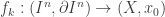

![\left[1-\frac{1}{2^{k-1}},1-\frac{1}{2^{k}}\right]\times I^{n-1}](https://s0.wp.com/latex.php?latex=%5Cleft%5B1-%5Cfrac%7B1%7D%7B2%5E%7Bk-1%7D%7D%2C1-%5Cfrac%7B1%7D%7B2%5E%7Bk%7D%7D%5Cright%5D%5Ctimes+I%5E%7Bn-1%7D&bg=ffffff&fg=333333&s=0&c=20201002)


Infinite product of 2-loops
By taking the homotopy class of 
![\{f_k\}_{k=1}^{\infty}\mapsto\left[\prod_{k=1}^{\infty}f_k\right]](https://s0.wp.com/latex.php?latex=%5C%7Bf_k%5C%7D_%7Bk%3D1%7D%5E%7B%5Cinfty%7D%5Cmapsto%5Cleft%5B%5Cprod_%7Bk%3D1%7D%5E%7B%5Cinfty%7Df_k%5Cright%5D&bg=ffffff&fg=333333&s=0&c=20201002)

Warning/Red Alert!! We may want to jump quickly to writing down a partially-defined infinite sum operation of homotopy classes by setting ![\sum_{k=1}^{\infty}[f_k]=\left[\prod_{k=1}^{\infty}f_k\right]](https://s0.wp.com/latex.php?latex=%5Csum_%7Bk%3D1%7D%5E%7B%5Cinfty%7D%5Bf_k%5D%3D%5Cleft%5B%5Cprod_%7Bk%3D1%7D%5E%7B%5Cinfty%7Df_k%5Cright%5D&bg=ffffff&fg=333333&s=0&c=20201002)
![\{[f_k]\}_{k=1}^{\infty}\mapsto\left[\prod_{k=1}^{\infty}f_k\right]](https://s0.wp.com/latex.php?latex=%5C%7B%5Bf_k%5D%5C%7D_%7Bk%3D1%7D%5E%7B%5Cinfty%7D%5Cmapsto%5Cleft%5B%5Cprod_%7Bk%3D1%7D%5E%7B%5Cinfty%7Df_k%5Cright%5D&bg=ffffff&fg=333333&s=0&c=20201002)


Here’s how infinite commutativity works for these particular kinds of infinite products:
Lemma: If 


Idea of the Proof. Let’s not do a technical proof here. Instead, let’s just see how this is done in pictures in dimension 


is homotopic to


Our pictures will look a lot like the Eckmann-Hilton gif from Part I but with infinitely many rectangles sliding around instead of just two. I’m afraid that I wasn’t ambitious enough to animate this so all you’ll get is a sequence of still images.
Throughout the following sequence of steps, the blue squares will represent the domain of the maps 


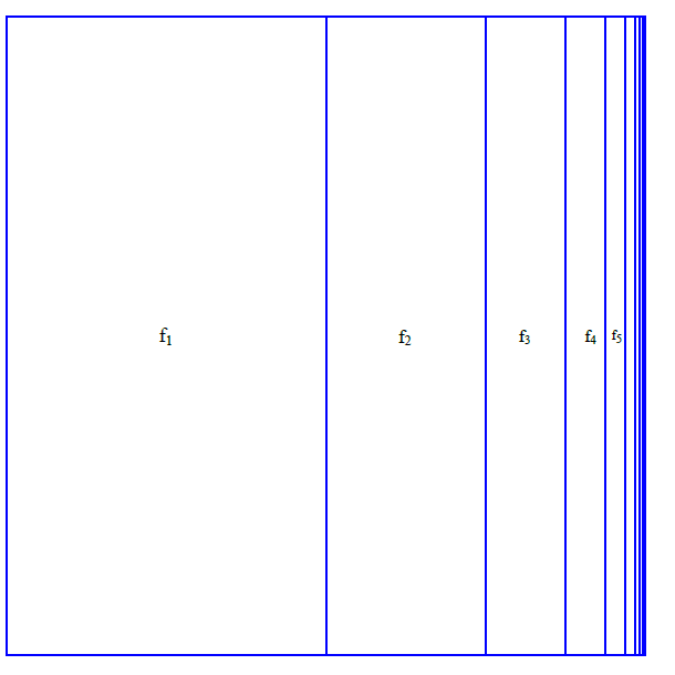
Now that we’ve done a vertical “reparameterization” we want to switch to a horizontal slide/stretch. This is where 


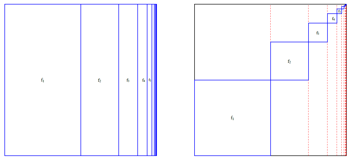
Now that we’ve taken care of things horizontally, it’s now a matter of some more vertical stretching to ensure that what we end up with is precisely an infinite product.

Finally, we end up with 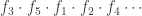

![H:[0,1]^3\to X](https://s0.wp.com/latex.php?latex=H%3A%5B0%2C1%5D%5E3%5Cto+X&bg=ffffff&fg=333333&s=0&c=20201002)

Eckmann Hilton Homotopy
Now imagine the same animation in this situation. There will be infinitely many cylinders ![S_1,S_2,S_3,...\subseteq [0,1]^3](https://s0.wp.com/latex.php?latex=S_1%2CS_2%2CS_3%2C...%5Csubseteq+%5B0%2C1%5D%5E3&bg=ffffff&fg=333333&s=0&c=20201002)
![[0,1]^3](https://s0.wp.com/latex.php?latex=%5B0%2C1%5D%5E3&bg=ffffff&fg=333333&s=0&c=20201002)


![[0,1]^3\backslash \bigcup_{k=1}^{\infty}int(S_k)](https://s0.wp.com/latex.php?latex=%5B0%2C1%5D%5E3%5Cbackslash+%5Cbigcup_%7Bk%3D1%7D%5E%7B%5Cinfty%7Dint%28S_k%29&bg=ffffff&fg=333333&s=0&c=20201002)


Hooray! We conclude that homotopy classes of infinite products in higher homotopy groups don’t change if you start shuffling around factors. So when infinite sums are well defined and the notation ![\sum_{k=1}^{\infty}[f_k]](https://s0.wp.com/latex.php?latex=%5Csum_%7Bk%3D1%7D%5E%7B%5Cinfty%7D%5Bf_k%5D&bg=ffffff&fg=333333&s=0&c=20201002)


Now you can imagine how this type of argument might be generalized and altered.
Definition: An n-domain is a (possibly infinite) collection 
![\prod_{m=1}^{n}[a_m,b_m]](https://s0.wp.com/latex.php?latex=%5Cprod_%7Bm%3D1%7D%5E%7Bn%7D%5Ba_m%2Cb_m%5D&bg=ffffff&fg=333333&s=0&c=20201002)
![[0,1]^n](https://s0.wp.com/latex.php?latex=%5B0%2C1%5D%5En&bg=ffffff&fg=333333&s=0&c=20201002)

The next step is to generalize the idea of infinite product to make sense for a general n-domain.
Definition: If 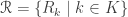


![[0,1]^n\backslash \bigcup_{k\in K}int(R_k)](https://s0.wp.com/latex.php?latex=%5B0%2C1%5D%5En%5Cbackslash+%5Cbigcup_%7Bk%5Cin+K%7Dint%28R_k%29&bg=ffffff&fg=333333&s=0&c=20201002)
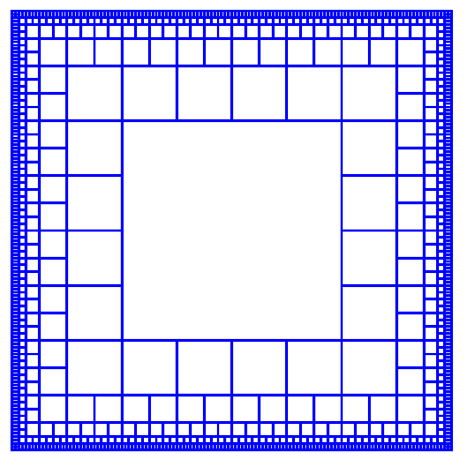
Be warned that n-domains are arbitrary.
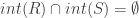
Some examples of 2-domains. Each rectangular region with a blue boundary is an element of the intended n-domain.
So the main question now is….
Question: Given any two n-domains 


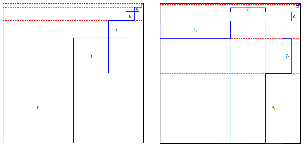
I can’t help but spoiling it… The answer is YES! This is a Theorem in [1]. Here’s why you should be even more startled that the answer is YES…The approach we took (in the lemma) for simultaneously sliding around individual squares/cubes fails miserably in general. It fails when you run into an n-domain that look like this:
Yikes! There’s no way to make individual moves and hope to shuffle them (after some choice of ordering) back into the simple n-domain for infinite products. If you try to move individual squares (all at once or even finitely many at a time), you will end up breaking continuity. Remember our original n-domain for defining ordinary infinite products (on the right)? How do you continuously shuffle the squares in the complicated one above to align with these ones, all of which have height 1? Aren’t we turning arbitrarily small things into big things???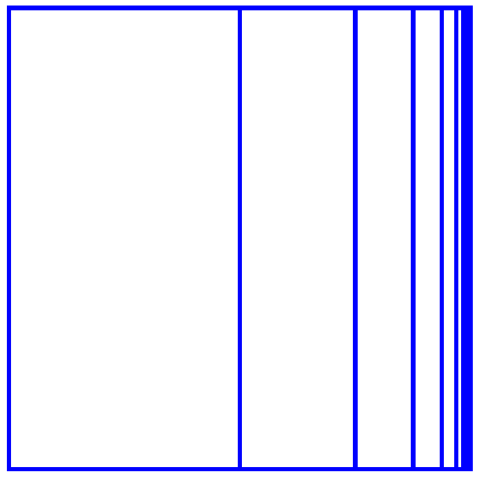
It seems like there’s just too much in the way and like sequences of squares that converge to the boundary are going to be a problem. Despite all this potential concern, there is a way to do it. Once you realize the main tricks, you have a ton of freedom to move things around in the domain while still holding a continuous homotopy in your hand at the end of the day. When I was writing the paper [1], I worked really hard to find the simplest geometric procedure I could possibly imagine to get the job done. The whole time, I was imagining these infinite swarms of rectangular cylinders twisting around each other in time just like the above gif with two cylinders. I had a lot of fun working it out and I am excited to see how this formalized interpretation of “infinite commutativity” will be applied.
So… not only are higher homotopy groups commutative for infinite products, they are commutative in this super-duper-geometric-infinite way.
A comment for operad fans
One cool thing here is the extension of the little 
For us infinitary-minded folks, we can take 
Just as 
References:
[1] J. Brazas, The infinitary n-cube shuffle. Topology Appl. 287 (2020) 107446. arXiv:2006.08738
[2] J. Brazas, P. Gillespie, Infinitary commutativity and abelianization in fundamental groups. (2020). To appear in the Journal of the Australian Math. Society.
[3] K. Eda, K. Kawamura, Homotopy and Homology Groups of the n-dimensional Hawaiian earring, Fund. Math. 165 (2000) 17-28.
[4] K. Kawamura, Low dimensional homotopy groups of suspensions of the Hawaiian earring, Colloq. Math. 96 (2003) no. 1 27-39.

Pingback: Infinite Commutativity: Part I | Wild Topology
Very nice post! I am having some trouble decoding some of the technical parts, and I wonder if you could set me straight if I’m fundamentally confused. Is the story essentially the following, at least in dimension 2?
The starting data is a null sequence of maps f_n of the unit disk, all of which map the boundary to the same point x.
The goal is to use the starting data to construct a single global map of the big unit disk E, and hope that any two reasonable constructions yield homotopic maps.
One way to do this is to start with a sequence of closed disks with disjoint interiors in E. Now use the map f_n to tell disk_n where to go. This is continuous, assumng the target space has reasonable properties. (Maybe it’s continuous even if the target does not have reasonable properties), this is more or less the pasting Lemma. Of course we map the complement of our disks to the special point.
So the hope is that any two maps of E build in this manner are homotopic? So is this story more or less the whole story? It is easy to be fooled in dimension 2. Does this story work the same way in all dimensions? (Actually maybe dimension 2 is more difficult, since it’s easier for the orbits of two of the small disks to collide under the purported homotopy). Thankyou for taking the time to read this.
LikeLike
Yes, for this post, that is the whole story. You have a null-sequence of based maps f_k:S^n\to X which, to compose, we view of as relative maps on [0,1]^n. Now take any sequence R_1,R_2,R_3,…of n-cubes with disjoint interiors in [0,1]^n. From this you can define a new map on f:S^n\to X which will be defined as f_k on R_k and maps everything else to the basepoint x. Like you mentioned, this is continuous no matter what the n-cubes look like because if U is any nbhd of x, then f^{-1}(U) will contain all but finitely many R_k (f_k was a null-sequence at x). The kicker is that if S_1,S_2,S_3,…is ANY other sequence of n-cubes with disjoint interiors (maybe some rearrangement of {R_k} or something completely unrelated like the complement of the Sierpinski carpet) and we define g to be f_k on S_k, then f and g will be homotopic! It works in all dimensions with exactly the same argument. Using sequences is just a convention I used to match up the factors f_k with which cube they should go with. The argument may seem a bit technical but it actually makes a lot of geometric sense once you’re willing to do some cube shrinking and start coming up with some clever cubical subdivisions. One key is not to go between arbitrary n-domains but rather to go from an arbitrary one to the standard sequence one.
Why do we need it to work for crazy, arbitrary configurations of squares/cubes? Well that is exactly what is required to characterize pi_n of the n-dimension Hawaiian earring and similar spaces. As I see it, this kind of general framework should be crucial for future work on pi_n.
LikeLike