Infinite Commutativity (Part I)

The Eckmann-Hilton Principle is a classical argument in algebraic topology/algebra. This argument allows you to conclude that an operation which may be expressed in two different ways (imagine that it may be applied both horizontally and vertically when written) is always commutative. This all has a very topological flavor that is important in homotopy theory. It is helpful to think of the two ways of expressing such an operation as having two-dimensions to move around in. This principle is fun to learn and revisit but it’s infinitary extension has become increasingly relevant in infinitary/wild topology. I’m spending a lot of time on the “elementary” Eckmann-Hilton homotopy in this post, because the infinite one in Part II is a fair bit more complicated and it will make a lot more sense if you remember how to “see” it.

The Algebraic Eckmann-Hilton Principle

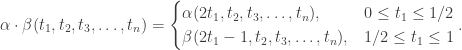
Here’s the set-up of the Eckmann-Hilton Principle: suppose you have a set $M$ with two unital operations $a\cdot b$ and $a\ast b$ satisfying the distributive rule: $(a\ast b)\cdot (c\ast d)=(a\cdot c)\ast (b\cdot d)$ . Using only this set-up, we have the following theorem.

Eckmann-Hilton Theorem: The operations $a\cdot b$ and $a\ast b$ are equal. Moreover, they are commutative and associative.

Proof. Let $e_{\cdot}$ and $e_{\ast}$ be the identity elements for the operations $\cdot$ and $\ast$ respectively. We check the desired equalities in sequence. Each argument uses a previous one.

Identities are equal:

$e_{\cdot}=e_{\cdot}\cdot e_{\cdot}=(e_{\cdot}\ast e_{\ast})\cdot (e_{\ast} \ast e_{\cdot})=(e_{\cdot}\cdot e_{\ast})\ast (e_{\ast}\cdot e_{\cdot})=e_{\ast}\ast e_{\ast}=e_{\ast}$

The operations agree:

$a\cdot b=(a \ast e_{\ast})\cdot (e_{\ast}\ast b)=(a\cdot e_{\ast})\ast (e_{\ast}\cdot b)=(a\cdot e_{\cdot})\ast (e_{\cdot}\cdot b)=a\ast b$

The operations are commutative:

$a\cdot b=(e_{\ast}\ast a)\cdot (b\ast e_{\ast})=( e_{\ast}\cdot b)\ast (a\cdot e_{\ast})=( e_{\cdot}\cdot b)\ast (a\cdot e_{\cdot})=b\ast a=b\cdot a$

Since the operation $\cdot$ is commutative and agrees with $\ast$ , the later is also commutative.

The operations are associative:

$a\cdot (b\cdot c)=(a\cdot e_{\cdot})\cdot (b\cdot c)=(a\cdot e_{\cdot})\ast (b\cdot c)=(a \ast b)\cdot (e_{\cdot} \ast c)=(a\cdot b)\cdot (e_{\ast} \ast c)=(a\cdot b)\cdot c$ . $\square$

The proof can be translated nicely into pictures if we transition to algebraic topology. For a based topological space $(X,x_0)$ , let $\Omega^n(X,x_0)$ be the set of all relative maps $(I^n,\partial I^n)\to (X,x_0)$ , which we call n-loops.

The Homotopical Eckmann-Hilton Principle

Given two n-loops $\alpha,\beta\in \Omega^n(X,x_0)$ , we can define the concatenation n-loop $\alpha\cdot\beta\in \Omega^n(X,x_0)$ by the formula:

$\alpha\cdot\beta(t_1,t_2,t_3,\dots,t_n)=\begin{cases} \alpha(2t_1,t_2,t_3,\dots,t_n), & 0\leq t_1\leq 1/2 \\ \beta(2t_1-1,t_2,t_3,\dots,t_n), & 1/2\leq t_1\leq 1 \end{cases} .$

Then $[\alpha]+[\beta]:=[\alpha\cdot\beta]$ defines the group operation of $\pi_n(X,x_0)$ . Let’s see why we can always commute $[\alpha]+[\beta]=[\beta]+[\alpha]$ . The following gif is basically a topological picture of the Eckmann-Hilton principle applied in dimension $n=2$ .

Slices of the commuting homotopy in dimension 2

In the animation, the the black boundaries and the gray shaded region are mapped to the basepoint $x_0\in X$ . The blue rectangle is the domain of $\alpha$ and the red rectangle is the domain of $\beta$ (with suitable scaling applied). The animation basically tells us how to define a homotopy from $\alpha\cdot\beta$ to $\beta\cdot\alpha$ as a map on a solid cube by showing how to define it on each vertical slice. Think of the start (height $t=0$ ) as mapping the bottom of a cube $[0,1]^3$ . It’s precisely $\alpha\cdot\beta$ . As time goes along, this animation realizes the how we want to map the cube into $X$ on higher slices $[0,1]^2\times\{t\}$ . Finally, the end ( $t=1$ ) is how we map the top of the cube as $\beta\cdot\alpha$ . Overall, we get a map on the cube, that is, a homotopy $H:[0,1]^2\times [0,1]\to X$ from $\alpha\cdot\beta$ to $\beta\cdot\alpha$ . Hence, $[\alpha]+[\beta]=[\alpha\cdot\beta]=[\beta\cdot\alpha]=[\beta]+[\alpha]$ .

It’s helpful for me to imagine what shape the red and blue squares will trace out in the cube $[0,1]^3$ . They look like cylinders with rectangle cross-sections that twist around each other in 3-space.

Commuting homotopy in dimension 2

This construction is one of the first things you learn when you start studying homotopy groups. It’s worth pointing out that this homotopy $\alpha\cdot\beta\simeq \beta\cdot\alpha$ has image in $Im(\alpha)\cup Im(\beta)$ and, in fact, has constant image for all “time” of the homotopy. In particular, you can commute small loops with small homotopies.

What is Infinite Commutativity?

Something quite remarkable is that as soon as we move up to the higher homotopy groups, things aren’t just commutative in the usual sense. The product operation on $\pi_n(X,x_0)$ , $n\geq 2$ turns out to be “infinitely commutative.” In Part II of this post, I’ll describe exactly what this means for homotopy groups. So, in the rest of the current post, I’m just going to try and give a simple answer to the question: what is an infinitary operation and what does it mean for it to be infinitely commutative?

If you’ve learned some abstract algebra, you know about binary operations and what it means to have a commutative binary operation. Typically, you’d end up with a commutative semigroup, monoid, group, ring, etc.

Definition: An infinitary operation on a set $X$ is a partially defined operation 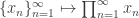$\{x_n\}_{n=1}^{\infty}\mapsto \prod_{n=1}^{\infty}x_n$ , which assigns an output (represented here using product notation) to certain infinite sequences in $X$ . It is also possible to index these products by sets other than the natural numbers $1,2,3,\dots$ . For example if $I$ is another indexing set (typically with an ordering or some other structure on it), then an infinitary $I$ -operation on $X$ is a partially defined operation $\{x_i\}_{i\in I}\mapsto \prod_{i\in I}x_i$ .

Of course, these kinds of operation can have a unit and you can impose axioms on them to express exactly how you’d like for them to be associative. The infinite sum/product operations I’m talking about here are not formal infinite sums. I’m interested in operations that are induced by topological limits and which extend familiar binary operations. Perhaps the most familiar one is the infinite sum operation on the real/complex numbers that you might learn about in Calculus or Analysis $\{x_n\}_{n=1}^{\infty}\mapsto \sum_{n=1}^{\infty}x_n$ . Chances are that if you’re reading this blog, you’ve seen these before.

Infinitary operations are all over the place, sometimes hiding in plain sight. Prominent examples include infinite sums, products related topological fields and rings of continuous functions on topological fields. Maybe a little less well-known are infinite compositions $f_1\circ f_2\circ f_3\circ\cdots$ and $\cdots \circ f_3\circ f_2\circ f_1$ which have applications to fixed point theory and number theory. There are analogous infinitary sum/product operations for matrices.

I hear that there are some folks who don’t enjoy working with actual topological spaces but like category theory. Well, I hate to break it to these folks but there is something implicitly topological about limits and colimits of infinite diagrams. Maybe in a future post I will clarify exactly how this is the case but I kind of describe how this goes in the introduction to this paper (published version [1]). Anyway, if $X_1\to X_2\to X_3\to\cdots$ is a directed system in a category and $X$ is the colimit of this diagram, then the canonical map $X_1\to X$ is very much the infinite composition $\cdots\circ f_3\circ f_2\circ f_1$ where $f_n:X_n\to X_{n+1}$ are the bonding maps. More generally, the canonical map $X_n\to X$ is the infinite composition $\cdots f_{n+2}\circ f_{n+1}\circ f_n$ . The dual situation works for inverse limits and you can replace the naturals $\omega$ with any well-ordered indexing set. Sometimes this kind of thing is called transfinite composition. The unavoidable topology that creeps in is hiding in the fact that the ordered set $X_1,X_2,X_3,\dots, X$ of objects (including the colimit) is indexed by a non-discrete compact ordered set, namely $\omega+1$ . It is not a coincidence that $\omega+1$ is order isomorphic to the set of cuts of $\omega$ .

Definition: An infinitary operation $\{x_n\}_{n=1}^{\infty}\mapsto \prod_{n=1}^{\infty}x_n$ on a set $X$ is infinitely commutative if for every bijection $\phi:\mathbb{N}\to\mathbb{N}$ , we have $\prod_{n=1}^{\infty}x_n=\prod_{n=1}^{\infty}x_{\phi(n)}$ .

For a more general $I$ -indexed operation, you would consider bijections $\phi:I\to I$ and demand that $\prod_{i\in I}x_i=\prod_{i\in I}x_{\phi(i)}$ always holds.

In short: Infinite commutativity means that you can permute the terms in the product in any way you like and the product will still be defined and its value will not change.

In fancy: Infinite commutativity means the natural action of the symmetric group $S_I$ of the indexing set on the $I$ -sequence $\{x_i\}_{i\in I}$ is invariant under the infinitary operation $\{x_i\}_{i\in I}\mapsto \prod_{i\in I}x_i$ .

Example: Even for infinite sums from Calculus, there are some subtleties involved. For instance, it is not enough to know the terms $a_1,a_2,a_3,...$ shrink to $0$ to ensure that $\sum_{n=1}^{\infty}a_n$ is well-defined, e.g. $1+\frac{1}{2}+\frac{1}{3}+\cdots$ diverges. Which sequences have a well-defined sum has more to do with the existence of a shrinking sequence of tails $t_n=a_n+a_{n+1}+a_{n+1}+\cdots$ as I described for infinite words. Also, there is a dichotomy of real infinite series: absolutely convergent series and conditionally convergent series. A series $\sum_{n=1}^{\infty}a_n$ is absolutely convergent if $\sum_{n=1}^{\infty}|a_n|$ converges and there is a Rearrangement Theorem stating that if $\phi:\mathbb{N}\to\mathbb{N}$ is any bijection then $\sum_{n=1}^{\infty}a_n= \sum_{n=1}^{\infty}a_{\phi(n)}$ . A series is conditionally convergent if it is not absolutely convergent and the Rearrangement Theorem states that if $\sum_{n=1}^{\infty}a_n$ is conditionally convergent and $L$ is any real number, then there exists a bijection $\phi$ such that $\sum_{n=1}^{\infty}a_{\phi(n)}=L$ . For instance, the alternating harmonic series $\sum_{n=1}^{\infty}\frac{(-1)^{n+1}}{n}=1-\frac{1}{2}+\frac{1}{3}-\frac{1}{4}+\cdots$ is conditionally convergent and its terms can be rearranged so the new sum converges to $42$ or $\pi$ or whatever number you want.

Takeaway: The infinite series operation in the real line is finitely commutative but is NOT infinitely commutative.

There are infinitary operations out there (like composition) which are not even finitely commutative. Here is one that is actually infinitely commutative.

Example: The Baer-Specker group $\mathbb{Z}^{\mathbb{N}}$ is the infinite direct product of discrete groups $\mathbb{Z}\times \mathbb{Z}\times\mathbb{Z}\times \cdots$ and consists of all infinite sequences of integers $\mathbf{a}=(a_1,a_2,a_3,\dots)$ . We give $\mathbb{Z}^{\mathbb{N}}$ the product topology so that a sequence of $\mathbf{a}_k=(a_{k,1},a_{k,2},a_{k,3},\dots)$ of sequences converges to $\mathbf{b}=(b_1,b_2,b_3,\dots)$ if and only if there initial coordinates in the sequence $\mathbf{a}_k$ stabilize to the terms of $\mathbf{b}$ , that is if for every $n\geq 1$ , there exists an $K\geq 1$ such that $a_{k,n}=b_n$ for all $k\geq K$ . So if you keep going through the sequence $\mathbf{a}_k$ , the first coordinate will eventually stabilize, then the second coordinate will eventually stabilize, and so on.

Now, given a sequence $\{\mathbf{a}_k\}_{k=1}^{\infty}\to (0,0,0,\dots)$ that converges to the identity, we can define a sum $\sum_{k=1}^{\infty}\mathbf{a}_k$ as the sequence

$\left(\sum_{k=1}^{\infty}a_{k,1},\sum_{k=1}^{\infty}a_{k,2},\sum_{k=1}^{\infty}a_{k,3},\dots \right)$

The infinite sum in each sequence is really just a finite sum since for given coordinate $n$ , the sequence $\{a_{k,n}\}_{n=1}^{\infty}$ is eventually $0$ .

Let’s check infinite commutativity. Suppose that $\phi:\mathbb{N}\to\mathbb{N}$ is a bijection. Then

$\sum_{k=1}^{\infty}\mathbf{a}_{\phi(k)}= \left(\sum_{k=1}^{\infty}a_{\phi(k),1},\sum_{k=1}^{\infty}a_{\phi(k),2},\sum_{k=1}^{\infty}a_{\phi(k),3},\dots \right)$

But each coordinate is just an ordinary finite sum. Hence, all that $\phi$ is really doing is commuting the finitely many non-zero terms in each coordinate. We can conclude that $\sum_{k=1}^{\infty}\mathbf{a}_k=\sum_{k=1}^{\infty}\mathbf{a}_{\phi(k)}$ , which means that the natural infinite sum operation on the Specker group is infinitely commutative. So, in an infinitary algebra sense, the Specker group is much simpler that the infinite series operation on the real line.

In Part II, we’ll explore why the natural infinitary operations on all higher homotopy groups are infinitely commutative!

[1] J. Brazas, Transfinite Product Reduction in Fundamental Groupoids. To Appear in European Journal of Mathematics. (2020). https://doi.org/10.1007/s40879-020-00413-0 arXiv version.

1 Response to Infinite Commutativity (Part I)

Pingback: Infinite Commutativity: Part II | Wild Topology