Understanding this post requires reading Part I where I explain what reduced paths are and how we might go about proving they exist. In this second part, I’ll go into detail about how to use Zorn’s lemma to identifying a maximal cancellation and therefore ensure every path is path-homotopic to a reduced path. The argument we’ll use is a generalization of Cannon and Conner’s [3, Theorem 3.9], which is based on Curtis and Fort’s original argument in [4, Lemma 3.1]. Both of those papers restrict only to one-dimensional spaces and here we’re going to include lots of other spaces using a definition introduced in [2]. While writing this post, I’ve been surprised at how far the argument can be generalized.
We’ll use the same notation as in Part I:  is a space,
 ![\alpha:[0,1]\to X](https://s0.wp.com/latex.php?latex=%5Calpha%3A%5B0%2C1%5D%5Cto+X&bg=ffffff&fg=333333&s=0&c=20201002) is a non-constant path, and
is a non-constant path, and  is the partially ordered set of cancellations of
  .
.
When can we be sure that pinching off null homotopic loops on a maximal cancellation results in a reduced loop?
At the start of Part I, I gave some examples of familiar spaces where some or all homotopy classes of loops failed to have any reduced representative. This means in order to continue this discussion, we must identify some hypothesis on that will allow us to move forward. The following definition has shown up in my work a good bit in the past two years. Curiously, it’s popping up again in a natural way. To distinguish notation, note that  denotes the fundamental group and
  denotes the fundamental groupoid.
Definition 8: A space has well-defined transfinite -products if for any closed set ![A \subseteq [0,1]](https://s0.wp.com/latex.php?latex=A+%5Csubseteq+%5B0%2C1%5D&bg=ffffff&fg=333333&s=0&c=20201002) containing
containing  and paths
 ![\alpha,\beta:[0,1]\to X](https://s0.wp.com/latex.php?latex=%5Calpha%2C%5Cbeta%3A%5B0%2C1%5D%5Cto+X&bg=ffffff&fg=333333&s=0&c=20201002) such that
such that  and
and ![\alpha|_{[a,b]}\simeq \beta|_{[a,b]}](https://s0.wp.com/latex.php?latex=%5Calpha%7C_%7B%5Ba%2Cb%5D%7D%5Csimeq+%5Cbeta%7C_%7B%5Ba%2Cb%5D%7D&bg=ffffff&fg=333333&s=0&c=20201002) for every component
for every component  of
of ![[0,1]\backslash A](https://s0.wp.com/latex.php?latex=%5B0%2C1%5D%5Cbackslash+A&bg=ffffff&fg=333333&s=0&c=20201002) , we have
, we have  .
.
This definition says that all infinite product operations ![\{[\alpha_j]\}_{j\in L}\mapsto \prod_{j\in L}[\alpha_j]](https://s0.wp.com/latex.php?latex=%5C%7B%5B%5Calpha_j%5D%5C%7D_%7Bj%5Cin+L%7D%5Cmapsto+%5Cprod_%7Bj%5Cin+L%7D%5B%5Calpha_j%5D&bg=ffffff&fg=333333&s=0&c=20201002) (indexed by any countable linear order
(indexed by any countable linear order  ) in the fundamental groupoid
  are well-defined on homotopy classes: homotopic factors result in homotopic products. For instance, in the case that
  , having well-defined transfinite products means that if we have path-homotopies
  ,
,  ,
,  ,… and we can form the infinite concatenations , then we have
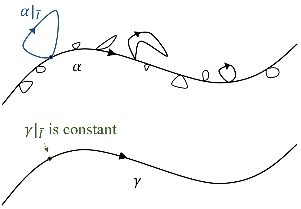
  (see the figure below). Why this is a hypothesis (and doesn’t just always happen for free) is because you may have no control over the size of the homotopies
  and you need them to shrink in order to form a continuous homotopy on the product.

If the space has well-defined infinite products (a special case of transfinite products) then if the top (blue) paths can be deformed into the bottom (red) paths individually, then the entire top path can be homotoped to the entire bottom path.
The set  in the definition could be the Cantor set, which means that we also need to consider the scenario in which the components of are densely ordered. That’s the worst case scenario, which is still not so bad, since there can only be countably many components. Spaces with well-defined transfinite -products abound, including one-dimensional spaces, planar sets, and lots of other spaces where “small null-homotopic loops are bounded by small disks.”
One remarkable thing about Definition 8 is that, for metrizable , this slightly-more-algebraic-flavored property is equivalent to admitting a generalized universal covering space . I haven’t had a chance to write about those yet, but they’re expected to be the primary tool for understanding wild higher homotopy groups.
Lemma 9 (Construction of reduced paths): Suppose has transfinite -products, is a path,  is a maximal cancellation for a and
 ![A=[0,1]\backslash\bigcup\mathscr{M}](https://s0.wp.com/latex.php?latex=A%3D%5B0%2C1%5D%5Cbackslash%5Cbigcup%5Cmathscr%7BM%7D&bg=ffffff&fg=333333&s=0&c=20201002) . If
. If ![\beta:[0,1]\to X](https://s0.wp.com/latex.php?latex=%5Cbeta%3A%5B0%2C1%5D%5Cto+X&bg=ffffff&fg=333333&s=0&c=20201002) is the path induced by a collapse function
is the path induced by a collapse function ![r:[0,1]\to[0,1]](https://s0.wp.com/latex.php?latex=r%3A%5B0%2C1%5D%5Cto%5B0%2C1%5D&bg=ffffff&fg=333333&s=0&c=20201002) for
for  , i.e.
  , then
  is reduced and .
Proof. Recall that since is maximal any two open intervals, which are elements of must have disjoint closures. Let ![A=[0,1]\backslash \bigcup\mathscr{M}](https://s0.wp.com/latex.php?latex=A%3D%5B0%2C1%5D%5Cbackslash+%5Cbigcup%5Cmathscr%7BM%7D&bg=ffffff&fg=333333&s=0&c=20201002) so that is the set of connected components of . Let
so that is the set of connected components of . Let ![\gamma:[0,1]\to X](https://s0.wp.com/latex.php?latex=%5Cgamma%3A%5B0%2C1%5D%5Cto+X&bg=ffffff&fg=333333&s=0&c=20201002) be the path, defined as on and constant on each element of (just like in the Pinching-off Lemma in Part I). If
be the path, defined as on and constant on each element of (just like in the Pinching-off Lemma in Part I). If  , then
 ![\alpha|_{[a,b]}](https://s0.wp.com/latex.php?latex=%5Calpha%7C_%7B%5Ba%2Cb%5D%7D&bg=ffffff&fg=333333&s=0&c=20201002) and
and ![\gamma|_{[a,b]}](https://s0.wp.com/latex.php?latex=%5Cgamma%7C_%7B%5Ba%2Cb%5D%7D&bg=ffffff&fg=333333&s=0&c=20201002) are both null-homotopic. So of course,
are both null-homotopic. So of course, ![\alpha|_{[a,b]}\simeq\gamma|_{[a,b]}](https://s0.wp.com/latex.php?latex=%5Calpha%7C_%7B%5Ba%2Cb%5D%7D%5Csimeq%5Cgamma%7C_%7B%5Ba%2Cb%5D%7D&bg=ffffff&fg=333333&s=0&c=20201002) . Therefore, since is assumed to have well-defined transfinite -products, we have
. Therefore, since is assumed to have well-defined transfinite -products, we have  . Now by Lemma 2 in Part I, we may find a collapse function
  for and a nowhere constant path such that
  . As pointed out in the comment after Lemma 2, we have
  . Therefore, .
Finally, we need to make sure that is reduced. Suppose to the contrary that there are  such that
 ![\beta|_{[c,d]}](https://s0.wp.com/latex.php?latex=%5Cbeta%7C_%7B%5Bc%2Cd%5D%7D&bg=ffffff&fg=333333&s=0&c=20201002) is a null-homotopic loop. Find
is a null-homotopic loop. Find ![c',d'\in A=[0,1]\backslash \bigcup\mathscr{M}](https://s0.wp.com/latex.php?latex=c%27%2Cd%27%5Cin+A%3D%5B0%2C1%5D%5Cbackslash+%5Cbigcup%5Cmathscr%7BM%7D&bg=ffffff&fg=333333&s=0&c=20201002) such that
such that  and
and  and
and  . Since
 ![\gamma|_{[c',d']}=\beta|_{[c,d]}\circ r|_{[c',d']}](https://s0.wp.com/latex.php?latex=%5Cgamma%7C_%7B%5Bc%27%2Cd%27%5D%7D%3D%5Cbeta%7C_%7B%5Bc%2Cd%5D%7D%5Ccirc+r%7C_%7B%5Bc%27%2Cd%27%5D%7D&bg=ffffff&fg=333333&s=0&c=20201002) , it must be that
, it must be that ![\gamma|_{[c',d']}](https://s0.wp.com/latex.php?latex=%5Cgamma%7C_%7B%5Bc%27%2Cd%27%5D%7D&bg=ffffff&fg=333333&s=0&c=20201002) is a null-homotopic loop. But remember that
is a null-homotopic loop. But remember that ![\alpha|_{[c',d']}](https://s0.wp.com/latex.php?latex=%5Calpha%7C_%7B%5Bc%27%2Cd%27%5D%7D&bg=ffffff&fg=333333&s=0&c=20201002) agrees with on
agrees with on ![[c',d']\backslash\bigcup\mathscr{M}](https://s0.wp.com/latex.php?latex=%5Bc%27%2Cd%27%5D%5Cbackslash%5Cbigcup%5Cmathscr%7BM%7D&bg=ffffff&fg=333333&s=0&c=20201002) and on any
and on any  that happens to lie in the interior of
 ![[c',d']](https://s0.wp.com/latex.php?latex=%5Bc%27%2Cd%27%5D&bg=ffffff&fg=333333&s=0&c=20201002) , is null-homotopic and
, is null-homotopic and  is constant. We once again apply the assumption that has well-defined transfinite -products to see that
 ![\alpha|_{[c',d']}\simeq\gamma|_{[c',d']}](https://s0.wp.com/latex.php?latex=%5Calpha%7C_%7B%5Bc%27%2Cd%27%5D%7D%5Csimeq%5Cgamma%7C_%7B%5Bc%27%2Cd%27%5D%7D&bg=ffffff&fg=333333&s=0&c=20201002) . Hence, is a null-homotopic loop. This allows us to define
. Hence, is a null-homotopic loop. This allows us to define ![\mathscr{M}'=\{(I\in\mathscr{M}\mid I\cap [c',d']=\emptyset\}\cup \{(c',d')\}](https://s0.wp.com/latex.php?latex=%5Cmathscr%7BM%7D%27%3D%5C%7B%28I%5Cin%5Cmathscr%7BM%7D%5Cmid+I%5Ccap+%5Bc%27%2Cd%27%5D%3D%5Cemptyset%5C%7D%5Ccup+%5C%7B%28c%27%2Cd%27%29%5C%7D&bg=ffffff&fg=333333&s=0&c=20201002) . Let’s see why this gives us a contradiction.
. Let’s see why this gives us a contradiction.
If there was no contained in  or if there is some such that
  is a proper subset of , then
  is a strictly larger cancellation than . This would violate the maximality of . Because
  , the only other possibility is that
  . However this would mean that
 ![r([c',d'])](https://s0.wp.com/latex.php?latex=r%28%5Bc%27%2Cd%27%5D%29&bg=ffffff&fg=333333&s=0&c=20201002) is a point, contradicting the assumption that
is a point, contradicting the assumption that  . Either way, we run into a problem. So it must be that is reduced.
Comment about understanding Lemma 9: Lemma 9 is packed with terminology from Part I so here’s how you can think about it. As long as has this well-defined products property, then given any maximal cancellation  , we can delete the subloops of defined on the components of (each of which is null-homotopic). I wrote the statement of Lemma 9 to avoid the case where itself is a null-homotopic loop. In that case, and won’t exist and you can always represent with the constant loop anyway.
When do maximal cancellations exist?
Ok, so this is the last piece of the puzzle and this is the one that requires Zorn’s Lemma. What we’re trying to do is start with a path and show that the partially ordered set of all cancellations of has a maximal element. So this is ripe for an application of Zorn’s Lemma, which is equivalent to the Axiom of Choice. You shouldn’t really expect this to work without Zorn’s lemma because maximal cancellations are not unique and very much are like choosing a contraction of a tree.
One again, the well-definedness property from Definition 9 is the natural hypothesis to complete the proof.
Lemma 10 (Existence of Maximal Cancellations): Suppose has well-defined transfinite -products and is a non-constant path. Then there exists a maximal cancellation for .
Proof. Let  be a linearly ordered subset of the partially ordered set . The result will follow from Zorn’s Lemma, if we can show that is bounded above in . Let
  . In otherwords, just union all of the open intervals together. Take be the set of connected components of
  . The main thing we’ll need to do is prove that is a cancellation. However, once this is done it’s not too hard to see that
  in for all
  .
.
The trickier part is showing that is a cancellation, i.e. that is a null-homotopic loop for all . Let’s fix such a connected component of . Notice that  . We need to pause and proof the following claim.
Claim: For every closed interval ![[c,d]\subseteq (a,b)](https://s0.wp.com/latex.php?latex=%5Bc%2Cd%5D%5Csubseteq+%28a%2Cb%29&bg=ffffff&fg=333333&s=0&c=20201002) , there exists a
, there exists a  and
and  such that
 ![[c,d]\subseteq (x,y)\subseteq (a,b)](https://s0.wp.com/latex.php?latex=%5Bc%2Cd%5D%5Csubseteq+%28x%2Cy%29%5Csubseteq+%28a%2Cb%29&bg=ffffff&fg=333333&s=0&c=20201002) .
.
Proof of Claim. Fix . For each ![t\in [c,d]](https://s0.wp.com/latex.php?latex=t%5Cin+%5Bc%2Cd%5D&bg=ffffff&fg=333333&s=0&c=20201002) , we have
, we have  and so there exists
  and
and  such that
  . Now
. Now ![\{I_t\mid t\in [c,d]\}](https://s0.wp.com/latex.php?latex=%5C%7BI_t%5Cmid+t%5Cin+%5Bc%2Cd%5D%5C%7D&bg=ffffff&fg=333333&s=0&c=20201002) is an open cover of the compact space
is an open cover of the compact space ![[c,d]](https://s0.wp.com/latex.php?latex=%5Bc%2Cd%5D&bg=ffffff&fg=333333&s=0&c=20201002) by open sets in and so we may find a finite subcover
by open sets in and so we may find a finite subcover  . Since
  is a linear order,
  exists. For
 ![s\in [c,d]](https://s0.wp.com/latex.php?latex=s%5Cin+%5Bc%2Cd%5D&bg=ffffff&fg=333333&s=0&c=20201002) , we have
, we have  for some
  and since
  , we have
  for some
  . We must have
  since .
Equipped with this now-proven Claim, we’re really going places. Start with some ![[c_1,d_1]\subseteq (a,b)](https://s0.wp.com/latex.php?latex=%5Bc_1%2Cd_1%5D%5Csubseteq+%28a%2Cb%29&bg=ffffff&fg=333333&s=0&c=20201002) . Find
. Find

such that  and
and  . Using the Claim, for every
  , we may find
  and
and  such that
 ![[c_n,d_n]\subseteq (x_n,y_n)\subseteq (a,b)](https://s0.wp.com/latex.php?latex=%5Bc_n%2Cd_n%5D%5Csubseteq+%28x_n%2Cy_n%29%5Csubseteq+%28a%2Cb%29&bg=ffffff&fg=333333&s=0&c=20201002) . This means that:
. This means that:


- Since each
 is a cancellation,
 ![\alpha|_{[x_n,y_n]}](https://s0.wp.com/latex.php?latex=%5Calpha%7C_%7B%5Bx_n%2Cy_n%5D%7D&bg=ffffff&fg=333333&s=0&c=20201002) is a null-homotopic loop!
is a null-homotopic loop!
Important early observation: Since the sequence  converges to both
  and
and  and we’ve assumed from the start that is Hausdorff, it must be the case that
  . All of the basepoints involved might be different but that’s ok… we’ll still work it out.
Define
![\gamma_m=\begin{cases} \alpha|_{[y_{m},y_{m+1}]} , &\text{ if }m\geq 1 \\ \alpha|_{[x_1,y_1]} , &\text{ if }m=0 \\ \alpha|_{[x_{-m-1},x_{-m}]}, &\text{ if }m\leq -1 \end{cases}](https://s0.wp.com/latex.php?latex=%5Cgamma_m%3D%5Cbegin%7Bcases%7D+%5Calpha%7C_%7B%5By_%7Bm%7D%2Cy_%7Bm%2B1%7D%5D%7D+%2C+%26%5Ctext%7B+if+%7Dm%5Cgeq+1+%5C%5C+%5Calpha%7C_%7B%5Bx_1%2Cy_1%5D%7D+%2C+%26%5Ctext%7B+if+%7Dm%3D0+%5C%5C+%5Calpha%7C_%7B%5Bx_%7B-m-1%7D%2Cx_%7B-m%7D%5D%7D%2C+%26%5Ctext%7B+if+%7Dm%5Cleq+-1+%5Cend%7Bcases%7D&bg=ffffff&fg=333333&s=0&c=20201002)
Warning: It is possible that  or
or  . In fact, we could have
  and/or
  for sufficiently large
  . To make sure that this proof doesn’t require a bunch of tedious cases, we allow
 ![\alpha|_{[p,q]}](https://s0.wp.com/latex.php?latex=%5Calpha%7C_%7B%5Bp%2Cq%5D%7D&bg=ffffff&fg=333333&s=0&c=20201002) to mean the constant loop at
to mean the constant loop at  when
when  .
.
Now, is homotopic to the  -indexed concatenation
  . At worst, we’re inserting a sequence of constant subpaths and reparameterizing, which never changes the path-homotopy class.

Now we go back and use that third bullet point. First, ![\gamma_0=\alpha|_{[x_1,y_1]}](https://s0.wp.com/latex.php?latex=%5Cgamma_0%3D%5Calpha%7C_%7B%5Bx_1%2Cy_1%5D%7D&bg=ffffff&fg=333333&s=0&c=20201002) is null-homotopic. Also, for
is null-homotopic. Also, for  , we have
 ![[\alpha|_{[x_{n+1},y_{n+1}]}]= [\gamma_{-n}][\alpha|_{[x_n,y_n]}][\gamma_{n}]](https://s0.wp.com/latex.php?latex=%5B%5Calpha%7C_%7B%5Bx_%7Bn%2B1%7D%2Cy_%7Bn%2B1%7D%5D%7D%5D%3D+%5B%5Cgamma_%7B-n%7D%5D%5B%5Calpha%7C_%7B%5Bx_n%2Cy_n%5D%7D%5D%5B%5Cgamma_%7Bn%7D%5D&bg=ffffff&fg=333333&s=0&c=20201002) where and
where and ![\alpha|_{[x_{n+1},y_{n+1}]}](https://s0.wp.com/latex.php?latex=%5Calpha%7C_%7B%5Bx_%7Bn%2B1%7D%2Cy_%7Bn%2B1%7D%5D%7D&bg=ffffff&fg=333333&s=0&c=20201002) are null-homotopic loops. Hence
are null-homotopic loops. Hence  for all .
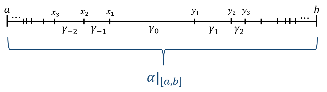
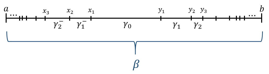
Define ![\beta:[a,b]\to X](https://s0.wp.com/latex.php?latex=%5Cbeta%3A%5Ba%2Cb%5D%5Cto+X&bg=ffffff&fg=333333&s=0&c=20201002) to be the loop, which is defined as
to be the loop, which is defined as  on
on ![[x_1,y_1]](https://s0.wp.com/latex.php?latex=%5Bx_1%2Cy_1%5D&bg=ffffff&fg=333333&s=0&c=20201002) ,
,  on
on ![[y_n,y_{n+1}]](https://s0.wp.com/latex.php?latex=%5By_n%2Cy_%7Bn%2B1%7D%5D&bg=ffffff&fg=333333&s=0&c=20201002) and
and  on
on ![[x_{n+1},x_{n}]](https://s0.wp.com/latex.php?latex=%5Bx_%7Bn%2B1%7D%2Cx_%7Bn%7D%5D&bg=ffffff&fg=333333&s=0&c=20201002) .
.

Notice that  is closed and and for every component latex of
 ![[a,b]\backslash A](https://s0.wp.com/latex.php?latex=%5Ba%2Cb%5D%5Cbackslash+A&bg=ffffff&fg=333333&s=0&c=20201002) , we have
, we have  . Therefore, since is assumed to have well-defined transfinite -products, we have
 ![\alpha|_{[a,b]}\simeq\beta](https://s0.wp.com/latex.php?latex=%5Calpha%7C_%7B%5Ba%2Cb%5D%7D%5Csimeq%5Cbeta&bg=ffffff&fg=333333&s=0&c=20201002) . However, is a reparemeterization of the path conjugate
. However, is a reparemeterization of the path conjugate  of the null-homotopic loop . Since is a null-homotopic loop, it follows that is null-homotopic.
Whew! Let’s put a little square here and be done with it.
An observation for those familiar with the Homotopically Hausdorff property: The well-defined transfinite products property is required when you run into densely ordered products. We really only needed products indexed by the naturals in the proof of Lemma 10. The subtleties of well-defined infinite path/loop products are studied in detail in [1] and are shown to be equivalent to the homotopically Hausdorff property when is first countable. So Lemma 10 could be strengthened as follows: Suppose is first countable and homotopically Hausdorff and is a non-constant path. Then there exists a maximal cancellation for .
Putting it all together
Finally, combining Lemmas 9 and 10, we finish off the existence of reduced paths.
Theorem 11: If has well-defined transfinite -products, then every path in is path-homotopic to a reduced path induced by deleting subloops on a maximal cancellation.
Proof. If is a null-homotopic loop, then the constant loop is the desired reduced representative. Otherwise, is a non-constant path. Lemma 10 ensures that contains a maximal cancellation . Lemma 9 ensures that if and is the path induced by a collapse function for (these details were laid out in Part I), then is reduced and .
What else is there to wonder about?
To what extent are reduced representatives of paths unique? In general, there is definitely no uniqueness within homotopy classes – recall the cylinder example from Part I. Even relative to the subloop deletion construction, the result won’t be unique. For suppose that ![\gamma_1,\gamma_2:[0,1]\to X](https://s0.wp.com/latex.php?latex=%5Cgamma_1%2C%5Cgamma_2%3A%5B0%2C1%5D%5Cto+X&bg=ffffff&fg=333333&s=0&c=20201002) are reduced paths that are path-homotopic to each other. Then
are reduced paths that are path-homotopic to each other. Then  , reduces to
  using the cancellation
  or
or  using the cancellation
  . There is choice involved! That choice will typically result in one of many possible reduced path results. This shouldn’t be too surprising though. It’s a slightly more topological version of the fact that in a group that is not free, shortest representation of an element using finite products of generators may not be unique.
However, I hinted in Part I that for one-dimensional spaces that every path-homotopy class has a unique (up to reparameterization) reduced path – I love this result. Maybe a Part III?
References:
[1] J. Brazas, Scattered products in fundamental groupoids. Proc. Amer. Math. Soc. 148 (2020), no 6, 2655-2670. arXiv
[2] J. Brazas, H. Fischer, Test map characterizations of local properties of fundamental groups. Journal of Topology and Analysis. 12 (2020) 37-85. arXiv
[3] J.W. Cannon, G.R. Conner, On the fundamental groups of one-dimensional spaces, Topology Appl. 153 (2006) 2648–2672.
[4] M.L. Curtis, M.K. Fort, Jr., The fundamental group of one-dimensional spaces, Proc. Amer. Math. Soc. 10 (1959) 140–148.


![[a,b]\subseteq [0,1]](https://s0.wp.com/latex.php?latex=%5Ba%2Cb%5D%5Csubseteq+%5B0%2C1%5D&bg=ffffff&fg=333333&s=0&c=20201002) such that
such that ![[0,1]^n\to X](https://s0.wp.com/latex.php?latex=%5B0%2C1%5D%5En%5Cto+X&bg=ffffff&fg=333333&s=0&c=20201002) should be for
should be for  ?
?![U\subseteq [0,1]](https://s0.wp.com/latex.php?latex=U%5Csubseteq+%5B0%2C1%5D&bg=ffffff&fg=333333&s=0&c=20201002) on which
on which ![[a,b]\subseteq U](https://s0.wp.com/latex.php?latex=%5Ba%2Cb%5D%5Csubseteq+U&bg=ffffff&fg=333333&s=0&c=20201002) such that
such that ![X=S^1\times [0,1]](https://s0.wp.com/latex.php?latex=X%3DS%5E1%5Ctimes+%5B0%2C1%5D&bg=ffffff&fg=333333&s=0&c=20201002) be the cylinder and for
be the cylinder and for ![z\in[0,1]](https://s0.wp.com/latex.php?latex=z%5Cin%5B0%2C1%5D&bg=ffffff&fg=333333&s=0&c=20201002) , consider the paths
, consider the paths  and
and  . Now the family of paths
  ,
, ![z\in [0,1]](https://s0.wp.com/latex.php?latex=z%5Cin+%5B0%2C1%5D&bg=ffffff&fg=333333&s=0&c=20201002) are all reduced paths that represent the same path-homotopy class. See the gif below.
are all reduced paths that represent the same path-homotopy class. See the gif below.

![S^1\times [0,1]](https://s0.wp.com/latex.php?latex=S%5E1%5Ctimes+%5B0%2C1%5D&bg=ffffff&fg=333333&s=0&c=20201002) is a 2-dimensional space (with whatever notion of topological dimension is your favorite).
is a 2-dimensional space (with whatever notion of topological dimension is your favorite). is the
  , then every non-trivial homotopy class
 ![1\neq [\alpha]\in \pi_1(\mathbb{G},b_0)](https://s0.wp.com/latex.php?latex=1%5Cneq+%5B%5Calpha%5D%5Cin+%5Cpi_1%28%5Cmathbb%7BG%7D%2Cb_0%29&bg=ffffff&fg=333333&s=0&c=20201002) has no reduced representative. This is true since every loop
has no reduced representative. This is true since every loop ![\gamma:[0,1]\to \mathbb{G}](https://s0.wp.com/latex.php?latex=%5Cgamma%3A%5B0%2C1%5D%5Cto+%5Cmathbb%7BG%7D&bg=ffffff&fg=333333&s=0&c=20201002) satisfying
satisfying  is null-homotopic in
  of inverse pairs you can delete the inverse pairs one-by-one or you could just delete them all at the same time. One difficulty we could face is that if
  is an infinite concatenation of null-homotopic loops, this product itself might not be null-homotopic. This phenomenon occurs precisely when the space in question fails to be
 ![r:[0,1]\to [0,1]](https://s0.wp.com/latex.php?latex=r%3A%5B0%2C1%5D%5Cto+%5B0%2C1%5D&bg=ffffff&fg=333333&s=0&c=20201002) and a nowhere constant path
and a nowhere constant path  .
.![t\in[0,1]](https://s0.wp.com/latex.php?latex=t%5Cin%5B0%2C1%5D&bg=ffffff&fg=333333&s=0&c=20201002) such that
such that  , i.e. there is an open neighborhood of
  be the connected components of
  , then
  must have disjoint closures. We give
 ![[0,1]](https://s0.wp.com/latex.php?latex=%5B0%2C1%5D&bg=ffffff&fg=333333&s=0&c=20201002) . For each
. For each  , pick a rational number
  . We define
  .
. in
in  , we use the linear function
  . Doing so adds the line segment connecting
  and
and  to the graph of
  yet, then
  in
in  . Therefore, we define
  .
. to be the dyadic rational that is the midpoint of
 such that
  . Since
  such that
  ,
,  , and
, and  . Now
. Now  and so we must have
  . By the definition of
  is a single point in
  . Thus
  , we have that
  . So, if we’re given a path
 ![A=[0,1]\backslash U](https://s0.wp.com/latex.php?latex=A%3D%5B0%2C1%5D%5Cbackslash+U&bg=ffffff&fg=333333&s=0&c=20201002) , then
, then ![r(A)=[0,1]](https://s0.wp.com/latex.php?latex=r%28A%29%3D%5B0%2C1%5D&bg=ffffff&fg=333333&s=0&c=20201002) .
.![A\subseteq [0,1]](https://s0.wp.com/latex.php?latex=A%5Csubseteq+%5B0%2C1%5D&bg=ffffff&fg=333333&s=0&c=20201002) is a closed set such that for each connected component
is a closed set such that for each connected component ![I\in C([0,1]\backslash A)](https://s0.wp.com/latex.php?latex=I%5Cin+C%28%5B0%2C1%5D%5Cbackslash+A%29&bg=ffffff&fg=333333&s=0&c=20201002) ,
,  is a loop, that is,
  to a single point. If
  for
for ![\gamma(t)=\begin{cases} \alpha(t), & \text{ if }t\in A\\ x_I, & \text{ if }t\in I, I\in C([0,1]\backslash A)\end{cases}](https://s0.wp.com/latex.php?latex=%5Cgamma%28t%29%3D%5Cbegin%7Bcases%7D+%5Calpha%28t%29%2C+%26+%5Ctext%7B+if+%7Dt%5Cin+A%5C%5C+x_I%2C+%26+%5Ctext%7B+if+%7Dt%5Cin+I%2C+I%5Cin+C%28%5B0%2C1%5D%5Cbackslash+A%29%5Cend%7Bcases%7D&bg=ffffff&fg=333333&s=0&c=20201002)

 of disjoint, connected open sets in
  , the subpath
  , we say
  if for every
  such that
  .
. is maximal if it is a maximal element of the partially ordered set
  .
. , then
 ![\alpha_{[a,c]}\simeq \alpha_{[a,b]}\cdot \alpha_{[b,c]}](https://s0.wp.com/latex.php?latex=%5Calpha_%7B%5Ba%2Cc%5D%7D%5Csimeq+%5Calpha_%7B%5Ba%2Cb%5D%7D%5Ccdot+%5Calpha_%7B%5Bb%2Cc%5D%7D&bg=ffffff&fg=333333&s=0&c=20201002) would be the concatenation of two null-homotopic loops and would therefore be null-homotopic. This would mean we could define
would be the concatenation of two null-homotopic loops and would therefore be null-homotopic. This would mean we could define  by replacing
  with
with  . This would give
  , violating the maximality of
  are one-dimensional Peano continua (connected, locally path-connected, compact metric spaces) and
  , then
  are homotopy equivalent. Why is this amazing? Because it includes spaces like the Hawaiian earring, double
  -tree “generalized” coverings (just like graphs have trees as universal covers) tells you that this is the case.
 is induced up to basepoint-change, that is, there exists a map
  and a path
 ![\beta:[0,1]\to Y](https://s0.wp.com/latex.php?latex=%5Cbeta%3A%5B0%2C1%5D%5Cto+Y&bg=ffffff&fg=333333&s=0&c=20201002) from
from  to
to  such that if
  ,
, ![\varphi_{\beta}([\alpha])=[\beta^{-}\cdot\alpha\cdot\beta]](https://s0.wp.com/latex.php?latex=%5Cvarphi_%7B%5Cbeta%7D%28%5B%5Calpha%5D%29%3D%5B%5Cbeta%5E%7B-%7D%5Ccdot%5Calpha%5Ccdot%5Cbeta%5D&bg=ffffff&fg=333333&s=0&c=20201002) is the basepoint-change isomorphism, then
is the basepoint-change isomorphism, then  .
.
 with the subspace topology is a homotopy invariant of
  , then
  . There is also a more algebraic version of this space, which I call the algebraic 1-wild set
  , which I contrast with
 is
is  is injective for all
  , then
  .
. is
is  , and, to obtain a contradiction, that
  . Then
  and so there exists a neighborhood
  of
of  such that
  , Given a loop
  is a loop in
  are homotopy inverses, then
  . Restricting the homotopies
  and
and  to
to ![\mathbf{w}(X)\times[0,1]](https://s0.wp.com/latex.php?latex=%5Cmathbf%7Bw%7D%28X%29%5Ctimes%5B0%2C1%5D&bg=ffffff&fg=333333&s=0&c=20201002) and
and ![\mathbf{w}(Y)\times [0,1]](https://s0.wp.com/latex.php?latex=%5Cmathbf%7Bw%7D%28Y%29%5Ctimes+%5B0%2C1%5D&bg=ffffff&fg=333333&s=0&c=20201002) respectively will show that the restrictions
respectively will show that the restrictions  and
and  are homotopy inverses.
 . This is an exceptionally useful rigidity result – if you want to deform the one-dimensional space in your hand, the wild points can’t go anywhere. Proving this requires knowing some special things about how loops can contract in one-dimensional spaces but the good news is that we can do everything we need to in this post without it.
 (with distinguished point
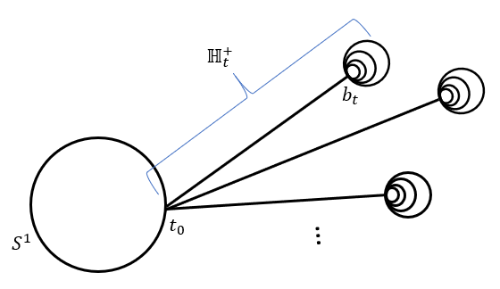
  ) and for every
  , let
, let  be a homeomorphic copy of the Hawaiian earring with basepoint
  . Now let
  . We give
  so that any compact subset of
 , we have
  with its usual topology.
 is a finite set, define
  . In other words,
  is the circle with finitely many earrings attached. The usual van Kampen Theorem shows that
  is the free product
  where the
  (this is the whole point of using the weak topology), it follows that
 is the thing we want. But actually, this won’t do because even when you take a one-point union
  of two first countable spaces where
  and
and  , the natural homomorphism
  is not an isomorphism because it’s not surjective. So we need to be a bit more careful not to attach wild points to each other.
![\mathbb{H}_{t}^{+}=\mathbb{H}_{t}\cup [0,1]/\mathord{\sim}](https://s0.wp.com/latex.php?latex=%5Cmathbb%7BH%7D_%7Bt%7D%5E%7B%2B%7D%3D%5Cmathbb%7BH%7D_%7Bt%7D%5Ccup+%5B0%2C1%5D%2F%5Cmathord%7B%5Csim%7D&bg=ffffff&fg=333333&s=0&c=20201002) ,
,  be the space obtained by attaching a “whisker” to the earring
  (the end of the whisker), denoted
  , to be the basepoint of
  .
. is now locally contractible at its basepoint so it’s now a good idea to consider the one-point union:
 .
.
 is homeomorphic to
  but I feel like doing this would just add confusion to the whole point of this.
 .
. and
and  .
. with it’s usual topology and
  that induces an isomorphism on fundamental groups. This makes sense since it’s possible to map the discrete circle continuously onto the usual circle. However, the above argument shows that no injective homomorphism
  can be induced by a map
  up to basepoint-change. A modification of these spaces could definitely be built so that an isomorphism is not induced in either direction.