Homotopically Reduced Paths (Part I)

The topic of this post focuses on a general concept that is heavily used in the wild topology world. Writing this post has been a fun exploration I’ve been meaning to spend time on for a while now. I will assume that all spaces involved are Hausdorff.

Definition 1: A path $\alpha:[0,1]\to X$ is (homotopically) reduced if either $\alpha$ is constant or if there is no interval $[a,b]\subseteq [0,1]$ such that $\alpha|_{[a,b]}$ is a null-homotopic loop, i.e. if $\alpha$ has no null-homotopic subloops.

I’ll usually just refer to a homotopically reduced path as a reduced path.

There are some other, more geometric, notions of “homotopically reduced” that are good for other purposes but this one is particularly relevant for one-dimensional spaces. Soon, we’ll combine new stuff with an old post to see that every path in a one-dimensional Hausdorff space is path-homotopic to a unique reduced path (unique up to reparameterization). Just as the uniqueness of reduced words in free groups is central to their theory and applications, the same kind of uniqueness for homotopy classes is important for proving things about fundamental groups of one-dimensional spaces.

History: The idea behind reduced paths in the one-dimensional case is based off of Curtis and Fort’s work in [2] from the 1950’s. I should note that Curtis-Fort use the notion of a “normal loop” which permits constant subpaths and is not exactly the same as in Definition 1. The modern definition of “reduced path,” which is far more effective for applications, does not permit constant subpaths. This modern version appears to appear first in Section 2 of Eda’s 2002 paper [3]. There is also a nice proof in Cannon and Conner’s outstanding 2006 paper [1].

Fun question to ponder: What do you think a homotopically reduced map $[0,1]^n\to X$ should be for $n\geq 2$ ?

Let’s start with some basic observations.

A homotopically reduced path $\alpha:[0,1]\to X$ that is not a constant path must be nowhere constant, i.e. there is no open set $U\subseteq [0,1]$ on which $\alpha$ is constant. For then we could find $[a,b]\subseteq U$ such that $\alpha|_{[a,b]}$ is the constant loop, which is null-homotopic.
In general, it’s possible for a path-homotopy class to be represented by many different reduced paths. For instance let $X=S^1\times [0,1]$ be the cylinder and for $z\in[0,1]$ , consider the paths $\ell_{z}(t)=\left(\cos(2 \pi t),\sin(2 \pi t),z\right)$ and $\mu_z(t)=(1,0,tz)$ . Now the family of paths $\mu_{z}\cdot \ell_{z}\cdot \mu_{z}^{-}$ , $z\in [0,1]$ are all reduced paths that represent the same path-homotopy class. See the gif below.
A family of reduced loops all representing the same homotopy class.

It’s worth pointing out that the cylinder $S^1\times [0,1]$ is a 2-dimensional space (with whatever notion of topological dimension is your favorite).
If $\mathbb{G}$ is the Griffiths twin cone with basepoint $b_0$ , then every non-trivial homotopy class $1\neq [\alpha]\in \pi_1(\mathbb{G},b_0)$ has no reduced representative. This is true since every loop $\gamma:[0,1]\to \mathbb{G}$ satisfying $\alpha^{-1}(b_0)=\{0,1\}$ is null-homotopic in $\mathbb{G}$ . You can start with any loop and begin pinching off null-homotopic subloops and you’ll never stop or arrive at a reduced loop. In fact it’s worse than that. No loop based at $b_0$ except for the constant loop will be reduced. Interestingly, only some elements of the fundamental group of the harmonic archipelago fail to have reduced representatives. Can you find one?

What I’d like to do in this post is discuss the existence of reduced paths in homotopy classes. When can we be sure that a path $\alpha:[0,1]\to X$ is path-homotopic to some reduced path?

Say we start with a non-constant path $\alpha$ . We want to “pinch off” or delete subloops which are null-homotopic loops. If you want to pinch things off one-by-one you’ll end up in an infinite deletion procedure, which could get pretty messy. So I think we should try to delete infinitely many subloops at a time. For example, if you have an infinite concatenation $\displaystyle\prod_{n=1}^{\infty}(\alpha_n\cdot\alpha_{n}^{-})$ of inverse pairs you can delete the inverse pairs one-by-one or you could just delete them all at the same time. One difficulty we could face is that if $\prod_{n=1}^{\infty}\alpha_n=\alpha_1\cdot\alpha_2\cdot\alpha_3\cdots$ is an infinite concatenation of null-homotopic loops, this product itself might not be null-homotopic. This phenomenon occurs precisely when the space in question fails to be homotopically Hausdorff, a concept very relevant to this post.

A Lemma about deleting constant subloops

Lemma 2: For every path $\alpha:[0,1]\to X$ , there exists a non-decreasing continuous function $r:[0,1]\to [0,1]$ and a nowhere constant path $\beta:[0,1]\to X$ such that $\beta\circ r=\alpha$ .

Proof. Let $U$ be the set of $t\in[0,1]$ such that $\alpha$ is locally constant at $t$ , i.e. there is an open neighborhood of $t$ on which $\alpha$ is constant. Let $C(U)$ be the connected components of $U$ and notice that if $I,J\in C(U)$ , then $I$ and $J$ must have disjoint closures. We give $C(U)$ the natural linear ordering inherited from $[0,1]$ . For each $I\in C(U)$ , pick a rational number $q_I\in I$ . We define $r$ as follows:

for each $I\in C(U)$ , we set $r(\overline{I})=q_I$ .
if $I=(a,b)<J=(c,d)$ in $C(U)$ are consecutive (no element of $C(U)$ is between them) then for $t\in (b,c)$ , we use the linear function $\displaystyle r(t)=\frac{q_J-q_I}{c-b}(t-b)+q_I$ . Doing so adds the line segment connecting $(b,q_I)$ and $(c,q_J)$ to the graph of $r$ .
If we haven’t defined $r(t)$ yet, then $t$ is the limit point of a monotone sequence of intervals $I_n$ in $C(U)$ , in the sense that $\{q_{I_n}\}\to t$ . Therefore, we define $r(t)=t$ .

A little real analysis will finish the proof that $r:[0,1]\to[0,1]$ is a well-defined, continuous, non-decreasing function. As a specific example, if $U$ is the complement of the middle-third Cantor set, and we choose the $q_I$ to be the dyadic rational that is the midpoint of $I$ . In this case, $r$ will be a modified version of the Cantor function.

The Cantor Function

In general, $r$ is always a kind of step function like the Cantor function that is constant on the components of $U$ .

Let’s finish this argument. Since $r$ is constant precisely on the components of $U$ . Since $r$ is a quotient map, and $\alpha$ is constant on the fibers of $r$ , there exists a unique map $\beta:[0,1]\to X$ such that $\beta\circ r=\alpha$ .

How do we know $\beta$ is nowhere constant? Suppose otherwise that there exists $a<b$ such that $\beta((a,b))=x\in X$ . Since $r$ is non-decreasing, continuous, and onto there exists $c<d$ such that $r(c)=a$ , $r(d)=b$ , and $r((c,d))=(a,b)$ . Now $\alpha((c,d))=\beta(r((c,d))=\beta((a,b))=x$ and so we must have $(c,d)\subseteq U$ . By the definition of $r$ , this means that $r((c,d))$ is a single point in $[0,1]$ , which contradicts $a<c$ . Thus $\beta$ cannot be constant on any open subset of $[0,1]$ . $\square$

Here’s why that lemma is a useful and necessary starting place: Since $\alpha=\beta\circ r$ , we have that $\alpha$ and $\beta$ are path-homotopic by the homotopy $H(s,t)=\beta(r(s)t+s(1-t))$ . So, if we’re given a path $\alpha$ , we can go ahead and delete a maximal family of constant subloops in one single step without changing the path-homotopy class. Hence, toward our goal for this post, we may assume from the start that $\alpha$ is nowhere constant.

But….to proceed we should dissect the proof to formalize the idea of “pinching off subloops.”

Definition 3: The function $r$ doesn’t need $\alpha$ to be constructed. In fact, given any open set $U$ in $[0,1]$ and the choice of a point in each connected component of $U$ , we can construct the function $r$ . We’ll refer to such a function as a collapse function for $U$ .

Notice that if $r$ is a collapse function for $U$ and $A=[0,1]\backslash U$ , then $r(A)=[0,1]$ .

Lemma 4 (Pinch-off Lemma): Suppose $\alpha:[0,1]\to X$ is a path and $A\subseteq [0,1]$ is a closed set such that for each connected component $I\in C([0,1]\backslash A)$ , $\alpha|_{\overline{I}}$ is a loop, that is, $\alpha$ maps the two points of $\partial I$ to a single point. If $r$ is a collapse function for $[0,1]\backslash A$ , then there exists path $\beta:[0,1]\to X$ such that $\beta\circ r|_{A}=\alpha|_{A}$ .

Proof. Suppose $\alpha(\partial I)=x_I$ for $I\in C(U)$ . Define an intermediate path $\gamma:[0,1]\to X$ so that

$\gamma(t)=\begin{cases} \alpha(t), & \text{ if }t\in A\\ x_I, & \text{ if }t\in I, I\in C([0,1]\backslash A)\end{cases}$

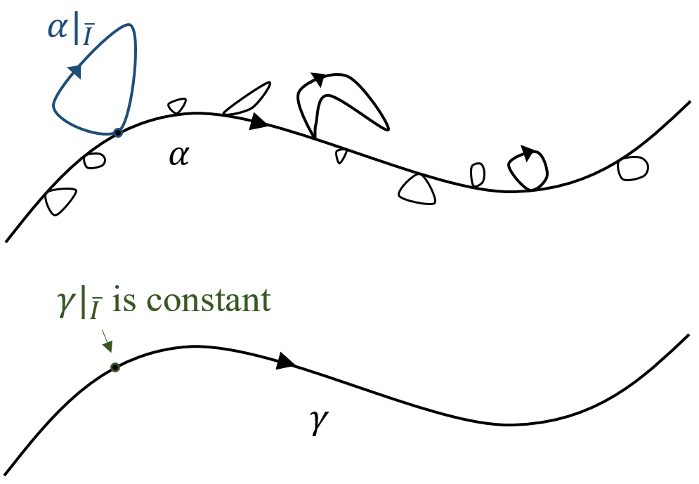
In other words, $\gamma$ is the same as $\alpha$ except that you force it to be constant on each component $I$ of $U$ .

Altering a path to be constant on a given (possibly infinite) family of subloops.

Because $\alpha$ is continuous, $\gamma$ is continuous. Moreover, $\gamma$ is now constant on each component of $U$ . Since $r$ is a quotient map and $\gamma$ is constant on the fibers of $r$ , there exists a unique path $\beta:[0,1]\to X$ such that $\beta\circ r=\gamma$ . Thus $\beta\circ r|_{A}=\gamma|_{A}=\alpha|_{A}$

Now this new pinch-off lemma is, in a way, much stronger than our first lemma. But we must be responsible with all this power. It just says that we can always pinch of subloops to obtain some continuous path. It doesn’t say that the result will be homotopic to the original….The resulting path will be “obviously” path-homotopic to the original only if we’re pinching off just finitely many null-homotopic subloops.

Maximal Cancellations

Definition 5: A cancellation of a path $\alpha$ is a collection $\mathscr{U}$ of disjoint, connected open sets in $[0,1]$ such that for each $I\in \mathscr{U}$ , the subpath $\alpha|_{\overline{I}}$ is a null-homotopic loop.

Let $\mathcal{C}(\alpha)$ be the set of all cancellations of $\alpha$ . Notice that $\mathcal{C}(\alpha)$ has a natural partial order: given $\mathscr{U},\mathscr{V}\in\mathcal{C}(\alpha)$ , we say $\mathscr{U}\leq \mathscr{V}$ if for every $I\in \mathscr{U}$ , there exists a $J\in \mathscr{V}$ such that $I\subseteq J$ .

Definition 6: A cancellation $\mathscr{M}\in \mathcal{C}(\alpha)$ is maximal if it is a maximal element of the partially ordered set $\mathcal{C}(\alpha),\leq)$ .

Observation 7: If $\mathscr{M}$ is a maximal cancellation of $\alpha$ , then the elements of $\mathscr{M}$ have disjoint closures. For if we have $(a,b),(b,c)\in \mathscr{M}$ , then $\alpha_{[a,c]}\simeq \alpha_{[a,b]}\cdot \alpha_{[b,c]}$ would be the concatenation of two null-homotopic loops and would therefore be null-homotopic. This would mean we could define $\mathscr{M}'\in\mathcal{C}(\alpha)$ by replacing $(a,b)$ and $(b,c)$ with $(a,c)$ . This would give $\mathscr{M}'>\mathscr{M}$ , violating the maximality of $\mathscr{M}$ .

So, we want to know two things:

When does a path $\alpha$ admit a maximal cancellation?
If $\alpha$ does admit a maximal cancellation $\mathscr{M}$ , and we form $\beta$ using a collapsing function $r$ for $\bigcup\mathscr{M}$ , must $\beta$ be path-homotopic to $\alpha$ ?

We’ll work to answer these questions in Part II.

References:

[1] J.W. Cannon, G.R. Conner, On the fundamental groups of one-dimensional spaces, Topology Appl. 153 (2006) 2648–2672.

[2] M.L. Curtis, M.K. Fort, Jr., The fundamental group of one-dimensional spaces, Proc. Amer. Math. Soc. 10 (1959) 140–148.

[3] K. Eda, The fundamental groups of one-dimensional spaces and spatial homomorphisms, Topology Appl. 123 (2002) no. 3, 479-505.

2 Responses to Homotopically Reduced Paths (Part I)

Pingback: Homotopically Reduced Paths (Part II) | Wild Topology
Pingback: Homotopically Reduced Paths (Part III) | Wild Topology