One of my posts where I did some substantial hand-waving is my original post on the fundamental group of the earring space. I wrote about how to understand and work with this group, but I never gave a proof of the key fact that the earring group naturally injects into an inverse limit of free groups  . This is one of the two primary viewpoints that researchers take to study and apply the beautiful algebra of this group (and more generally fundamental groups of one-dimensional spaces). Seriously, I’m using this machinery like 1.) it’s going out of style and 2.) I understand fashion. The other approach avoids inverse limits by identifying the earring group as a group of reduced countable, linear words over a countable alphabet. They’re logically equivalent, but sometimes one is more convenient than the other.
To be honest, I hesitated about writing this post. I say with confidence that there is no completely elementary proof. While I’ve read and understood many different proofs of shape injectivity, most of them are either super technical or they gloss over details by applying continuum and dimension theory. Some inquisitive and kind readers have given me the motivation to do it.
When trying to write this post, I dug deep into the literature trying to weasel out an almost entirely self-contained proof that a grad student would believe. After some reading, I worked things out and these posts are the results of the effort. This first post will mostly be used to set up the technical tools about arcs in inverse limits that we’ll need to prove shape injectivity.
Let  be the circle of radius
  centered at
  . Then
  is the earring with basepoint
  . We need to set up a little more notation:
- Let
 be the bouquet of the first n-circles with free fundamental group
  .
.
- Let
 be the retraction, which collapses
  to
to  and is the identity elsewhere.
- Let
 be the retraction, which collapses the smaller copy of the earring
  to and is the identity elsewhere.
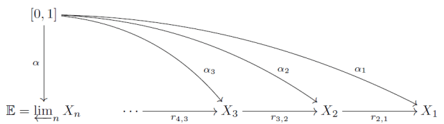
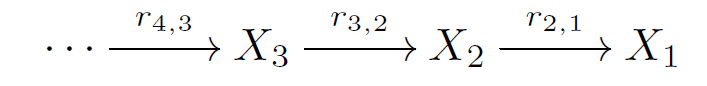
This gives an inverse system of retracts:


The closed mapping theorem should help convince you that the earring is homeomorphic to the inverse limit of this system of bouquets. Now apply  to this inverse system: the maps induce homomorphisms
  , which together induce a canonical homomorphism
  defined by
 ![\phi([\alpha])=([r_1\circ\alpha],[r_2\circ\alpha],[r_3\circ\alpha],\dots)](https://s0.wp.com/latex.php?latex=%5Cphi%28%5B%5Calpha%5D%29%3D%28%5Br_1%5Ccirc%5Calpha%5D%2C%5Br_2%5Ccirc%5Calpha%5D%2C%5Br_3%5Ccirc%5Calpha%5D%2C%5Cdots%29&bg=ffffff&fg=333333&s=0&c=20201002) .
.

The inverse limit of free groups, which we can abbreviate as is precisely the first shape (or Cech) homotopy group  .
.
First, let’s notice that  is homeomorphic to
  . Basically, we just need to believe that is precisely the infinite wedge
  viewed as a subspace of the infinite torus
  with the product topology. It’s then very tempting to think that
  is an isomorphism. However, doesn’t always preserve inverse limits!
Nevertheless, we can still understand and work with  if we identify it as a subgroup of . Hence, the motivation for showing that is injective.
Shape Injectivity Theorem: is injective.
Basically, this theorem says that a loop  in is null-homotopic if and only if every projection
  is null-homotopic in the wedge of circles
  . The contrapositive says that is not null-homotopic in iff there exists some
  such that represents a non-trivial word in
  .
.
Why this is not so obvious
Let  be the loop going once around
  counterclockwise and let
  be its reverse loop. Given a loop
 ![\alpha:[0,1]\to\mathbb{E}](https://s0.wp.com/latex.php?latex=%5Calpha%3A%5B0%2C1%5D%5Cto%5Cmathbb%7BE%7D&bg=ffffff&fg=333333&s=0&c=20201002) , we may assume that for each component
, we may assume that for each component  of
of ![[0,1]\backslash\alpha^{-1}(b_0)](https://s0.wp.com/latex.php?latex=%5B0%2C1%5D%5Cbackslash%5Calpha%5E%7B-1%7D%28b_0%29&bg=ffffff&fg=333333&s=0&c=20201002) , the restriction of to
, the restriction of to ![[a,b]](https://s0.wp.com/latex.php?latex=%5Ba%2Cb%5D&bg=ffffff&fg=333333&s=0&c=20201002) is one of the paths or . Obviously, for each , the loops
is one of the paths or . Obviously, for each , the loops  and can show up as subloops at most finitely many times or we would violate the uniform continuity of .
Suppose we know is null-homotopic in . The primary difficulty is that the null-homotopies ![H_n:[0,1]^2\to X_n](https://s0.wp.com/latex.php?latex=H_n%3A%5B0%2C1%5D%5E2%5Cto+X_n&bg=ffffff&fg=333333&s=0&c=20201002) for might have nothing to do with each other. We just know one exists for each approximation level. There is no guarantee that we can “fix em up right” so that they agree with the bonding maps, i.e. satisfy
for might have nothing to do with each other. We just know one exists for each approximation level. There is no guarantee that we can “fix em up right” so that they agree with the bonding maps, i.e. satisfy  and thus induce a null-homotopy of in
  .
.
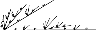
Here is a more algebraic way to look at it. It doesn’t hurt to think each projection loop as an unreduced finite word in the letters  . Then
  means a concatenation
  of length
  and
and  means a concatenation
  of length . For instance, suppose is the loop described by the following projections.


- and so on where between any two letters in the previous projection you insert an inverse pair of the form
 .
.
Notice that deleting the  ‘s from
  gives
gives  , deleting the
  ‘s from
  gives , and so on. Moreover, each letter is only used finitely many times. We conclude that this does indeed give a loop in . Notice that even though these finite projection words are getting pretty long, the homotopy class
 ![[r_n\circ\alpha]](https://s0.wp.com/latex.php?latex=%5Br_n%5Ccirc%5Calpha%5D&bg=ffffff&fg=333333&s=0&c=20201002) will cancel to the trivial word in the free group . After all, we just inserted inverse pairs that cancel!
will cancel to the trivial word in the free group . After all, we just inserted inverse pairs that cancel!
But the infinite limit loop in is a “transfinite word” of dense order. It is null-homotopic (due to the main result of the post) but it’s much harder to come up with an explicit contraction because there is no finite reduction scheme that can do the job. Between any two of the inverse pairs that you wanted to cancel in the n-th projection, you actually had letters  up in the next level. You can’t just cancel in the
  -th level, forget about what you just did, and then move on up to the
  -st level.
The trouble is that the process of cancellation requires choice. Ok, there’s not much choice in cancelling the first word. But look at the second one.
You could cancel all the ‘s first and then the remaining  ‘s. Or you could cancel the middle ‘s first, then the ‘s, and then the remaining ‘s. It may not seem like a big deal but these are different homotopies! The only thing we have going for us it that we have some contracting reduction for each . This leaves us with an infinite sequence of reductions for the projection words – one for each level. We have no idea if these reductions match up or can be chosen so that the projection of a reduction of to the next level down is exactly the reduction for
 ![[r_{n-1}\circ\alpha]](https://s0.wp.com/latex.php?latex=%5Br_%7Bn-1%7D%5Ccirc%5Calpha%5D&bg=ffffff&fg=333333&s=0&c=20201002) . Sure, once I choose a reduction/null-homotopy for , I can project it down to make sure the reductions on lower levels match up, but then you have to start over and worry about
. Sure, once I choose a reduction/null-homotopy for , I can project it down to make sure the reductions on lower levels match up, but then you have to start over and worry about ![[r_{n+1}\circ\alpha]](https://s0.wp.com/latex.php?latex=%5Br_%7Bn%2B1%7D%5Ccirc%5Calpha%5D&bg=ffffff&fg=333333&s=0&c=20201002) . If you project down and fix all the lower levels and continue this process all the way up, you’re going to end up with a rearranging the reduction choice at each level infinitely many times. There is no guarantee this can be done “continuously.”
. If you project down and fix all the lower levels and continue this process all the way up, you’re going to end up with a rearranging the reduction choice at each level infinitely many times. There is no guarantee this can be done “continuously.”
History
The first attempt to identify was by H.B. Griffiths [3]. However, there was a critical error in Griffiths’ proof of the injectivity. The error was observed and a correct proof finally given (30 years later!) by Morgan and Morrison [4]. Many years back when I read the original proof for the first time, I was a bit unsatisfied with how specific and technical it all was. Later on, I read the proof given by Eda and Kawamura in [2], which felt more intuitive because all I had to do was understand inverse limits and believe a little continuum theory. Bonus: It applies to all spaces with Lebesgue covering dimension 1, not just . The key idea is originally due to the work in [1] by Curtis and Fort from the 1950’s.
Trees and Inverse Limits
An important theme in wild topology is the idea of a space being “uniquely arc-wise connected.” Here an “arc” in a space refers to a subspace of homeomorphic to ![[0,1]](https://s0.wp.com/latex.php?latex=%5B0%2C1%5D&bg=ffffff&fg=333333&s=0&c=20201002) . The image of
. The image of  and
and  in are the endpoints of the arc. A “simple closed curve” in is a homeomorphic copy of the unit circle
  .
.
Definition: A space is uniquely arc-wise connected if for all distinct points  , there is a unique arc in whose endpoints are
  and
and  .
.
The next proposition gives another useful way to describe uniquely arc-wise connected spaces.
Proposition: If is uniquely arc-wise connected, then is path connected and contains no simple closed curves. The converse holds if is weakly Hausdorff.
Proof. Since is not uniquely arc-wise connected, one direction is obvious. Now suppose is weakly Hausdorff and not uniquely arc-wise connected. Then there are distinct arcs  sharing the same endpoints. Since
  , without loss of generality, we may suppose there is a point
  . Note that since is weakly Hausdorff,
  and
and  are closed. It follows that
  is non-empty and closed in and thus
  is open in . Choosing a homeomorphism
 ![h: [0,1]\to A](https://s0.wp.com/latex.php?latex=h%3A+%5B0%2C1%5D%5Cto+A&bg=ffffff&fg=333333&s=0&c=20201002) , let
, let  be the component of
  containing
  . Now
. Now ![A_1=h([c,d])](https://s0.wp.com/latex.php?latex=A_1%3Dh%28%5Bc%2Cd%5D%29&bg=ffffff&fg=333333&s=0&c=20201002) is a subarc of with endpoints
is a subarc of with endpoints  . If
. If  is the subarc of with endpoints
  and
and  , then we have
  . Now it’s clear that
  is a homeomorphic image of a circle, i.e. a simple closed curve.
The uniquely arc-wise connected spaces you’re most likely to already be familiar with are trees.
Definition: A simplicial tree is a one-dimensional simplicial complex without any cycles. A (topological) tree is a space, which is the geometric realization of a simplicial tree.
Basic algebraic topology tells us that trees are contractible and uniquely arc-wise connected. Since a tree  is simply connected, between any two points
  there is a single homotopy (rel. endpoints) class of paths from to . This means
 ![\beta:[0,1]\to T](https://s0.wp.com/latex.php?latex=%5Cbeta%3A%5B0%2C1%5D%5Cto+T&bg=ffffff&fg=333333&s=0&c=20201002) of the unique arc from to is a reduced representative of the single homotopy class of paths from to in the sense that it has no null-homotopic subloops. This reduced representative is unique up to reparameterization. A non-reduced path in a tree would have some null-homotopic zig-zags that we could “delete” by a homotopy to obtain a reduced representative. Of course, there could be infinitely many zig-zags but since trees are semilocally simply connected, this is not much of an obstacle to overcome.
of the unique arc from to is a reduced representative of the single homotopy class of paths from to in the sense that it has no null-homotopic subloops. This reduced representative is unique up to reparameterization. A non-reduced path in a tree would have some null-homotopic zig-zags that we could “delete” by a homotopy to obtain a reduced representative. Of course, there could be infinitely many zig-zags but since trees are semilocally simply connected, this is not much of an obstacle to overcome.
Now what about an inverse limit  of trees
  ? Informally, such an inverse limit “glues” together the trees according to their bonding maps. The result should be one-dimensional and if
  maps
maps  to the same point of , then will send the unique arc connecting and to a finite topological subtree of . So there should be no way for a simple closed curve to magically appear in the gluing process. We’ll prove exactly this using the simplest proof I could come up with.
Recall that an inverse limit  is topologized as a subspace of
  . If
. If  are the projection maps, then a point
  is represented by the sequence
  . A basic open neighborhood latex of is of the form
  where
where  is an open neighborhood of
  and there is an
  such that
  for
for  . Since the functions are continuous and
  , we may replace
  with
with  where
where  . Terminating at
  , we can inductively replace with
  where
where  . In this way, we may take a basic open neighborhood of to satisfy
  for
for  and for .
Lemma: Suppose  is an inverse limit of Hausdorff spaces and are the projection maps. If
  are disjoint compact subsets of , then there exists an such that
  .
.
Proof. Suppose, to obtain a contradiction, that for every there exists  and
and  such that
  . Notice that since the coordinates of each
  and
and  must agree with the bonding maps , this means
  for all
  . Since and are compact, we may find a subsequences
  and
and  that converge to
  and
and  respectively. We’re going to prove that also converges to
  . Consider a basic open neighborhood
  of . Let
  be the minimal such that
  . Since
  , there exists a
  such that
  for all
  . We can choose
  large enough so that
  . Now pick any . Since
  , we have
  for all
  . Since
  , this implies that
  for
for  . Hence
  (for ) and we conclude that
  . However, this means the converges to both of the points and
  ; an impossibility in a Hausdorff space.
Remark: Notice that if  , then it must also be the case that
  for
for  . So for given and , we can choose to be as large as we want.
Theorem: An inverse limit  of trees contains no simple closed curves.
Proof. Since topological trees are always Hausdorff, is Hausdorff. Suppose, to obtain a contradiction, that  is an embedding. For
  , let
, let  be the intersection of and
  -th quadrant of the plane (include the bounding axes). Now
  are four (compact) arcs in the meet at endpoints to form the simple closed curve
  . Let
. Let  and
and  . Notice that
  and
and  . Let
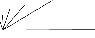
. Let  be the paths that trace the arcs
  with the orientation shown below so that
  and
and  are injective paths from to .

According to the previous Lemma (and the following Remark), if we denote the projection maps by  , then we can find an such that
  and
and  . Note that
  and
and  are distinct points in the tree
  (as
(as  and
and  are disjoint) and are thus connected in by a unique arc. Let
 ![\beta:[0,1]\to X](https://s0.wp.com/latex.php?latex=%5Cbeta%3A%5B0%2C1%5D%5Cto+X&bg=ffffff&fg=333333&s=0&c=20201002) trace out this arc from to . Now
trace out this arc from to . Now  is the reduced representative of both
  and
and  .
.
- Considering the reduction of the path
 to , we see that an initial segment
 ![\beta|_{[0,s]}](https://s0.wp.com/latex.php?latex=%5Cbeta%7C_%7B%5B0%2Cs%5D%7D&bg=ffffff&fg=333333&s=0&c=20201002) has image in and the terminal segment
has image in and the terminal segment ![\beta|_{[s,1]}](https://s0.wp.com/latex.php?latex=%5Cbeta%7C_%7B%5Bs%2C1%5D%7D&bg=ffffff&fg=333333&s=0&c=20201002) has image in
has image in  .
.
- Considering the reduction of the path
 to , we see that an initial segment
 ![\beta|_{[0,t]}](https://s0.wp.com/latex.php?latex=%5Cbeta%7C_%7B%5B0%2Ct%5D%7D&bg=ffffff&fg=333333&s=0&c=20201002) has image in
has image in  and the terminal segment
 ![\beta|_{[t,1]}](https://s0.wp.com/latex.php?latex=%5Cbeta%7C_%7B%5Bt%2C1%5D%7D&bg=ffffff&fg=333333&s=0&c=20201002) has image in .
has image in .
- If
 , then
 ![\beta([s,t])\subset f_m(A_2)\cap f_m(A_4)](https://s0.wp.com/latex.php?latex=%5Cbeta%28%5Bs%2Ct%5D%29%5Csubset+f_m%28A_2%29%5Ccap+f_m%28A_4%29&bg=ffffff&fg=333333&s=0&c=20201002) .
.
- If
 , then
 ![\beta([t,s])\subseteq f_m(A_1)\cap f_m(A_3)](https://s0.wp.com/latex.php?latex=%5Cbeta%28%5Bt%2Cs%5D%29%5Csubseteq+f_m%28A_1%29%5Ccap+f_m%28A_3%29&bg=ffffff&fg=333333&s=0&c=20201002) .
.
- If
 , then
  lies in every
  .
.
In any of these cases, even the degenerate ones where one of  or
or  is or , we arrive at a contradiction.
Corollary: Every path-component of the limit of an inverse system of trees is uniquely arc-wise connected.
In Part II, the fact that an inverse limit of trees contains no simple closed curves will be a critical part of proving the Shape Injectivity Theorem.
References.
[1] M.L. Curtis and M.K. Fort, The fundamental group of one-dimensional spaces, Proc. Amer. Math. Soc. 10 (1959) 140-148.
[2] K. Eda and K. Kawamura, The fundamental groups of one-dimensional spaces, Topology and its Applications 87 (1998) 163-172.
[3] H.B. Griffiths, Infinite products of semigroups and local connectivity, Proc. London Math. Soc. (3), 6 (1956), 455-485.
[4] J.W. Morgan and I. Morrison, A van Kampen theorem for weak joins, Proceedings of the London Mathematical Society 53 (1986) 562-576.


![[0,1]\to X](https://s0.wp.com/latex.php?latex=%5B0%2C1%5D%5Cto+X&bg=ffffff&fg=333333&s=0&c=20201002)


![T_1=[0,1]](https://s0.wp.com/latex.php?latex=T_1%3D%5B0%2C1%5D&bg=ffffff&fg=333333&s=0&c=20201002)


![i_{x,y}:[0,d(x,y)]\to D](https://s0.wp.com/latex.php?latex=i_%7Bx%2Cy%7D%3A%5B0%2Cd%28x%2Cy%29%5D%5Cto+D&bg=ffffff&fg=333333&s=0&c=20201002)


![H:D\times [0,1]\to D](https://s0.wp.com/latex.php?latex=H%3AD%5Ctimes+%5B0%2C1%5D%5Cto+D&bg=ffffff&fg=333333&s=0&c=20201002)


![\phi([\alpha])=([r_1\circ\alpha],[r_2\circ\alpha],\dots)](https://s0.wp.com/latex.php?latex=%5Cphi%28%5B%5Calpha%5D%29%3D%28%5Br_1%5Ccirc%5Calpha%5D%2C%5Br_2%5Ccirc%5Calpha%5D%2C%5Cdots%29&bg=ffffff&fg=333333&s=0&c=20201002)

![\alpha:[0,1]\to \mathbb{E}](https://s0.wp.com/latex.php?latex=%5Calpha%3A%5B0%2C1%5D%5Cto+%5Cmathbb%7BE%7D&bg=ffffff&fg=333333&s=0&c=20201002)
![r_n\circ\alpha:[0,1]\to X_n](https://s0.wp.com/latex.php?latex=r_n%5Ccirc%5Calpha%3A%5B0%2C1%5D%5Cto+X_n&bg=ffffff&fg=333333&s=0&c=20201002)


![\alpha_n=r_n\circ\alpha:[0,1]\to X_n](https://s0.wp.com/latex.php?latex=%5Calpha_n%3Dr_n%5Ccirc%5Calpha%3A%5B0%2C1%5D%5Cto+X_n&bg=ffffff&fg=333333&s=0&c=20201002)

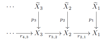
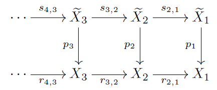
![\widetilde{\alpha}_n:([0,1],0)\to (\widetilde{X}_n,\widetilde{x}_n)](https://s0.wp.com/latex.php?latex=%5Cwidetilde%7B%5Calpha%7D_n%3A%28%5B0%2C1%5D%2C0%29%5Cto+%28%5Cwidetilde%7BX%7D_n%2C%5Cwidetilde%7Bx%7D_n%29&bg=ffffff&fg=333333&s=0&c=20201002)


![\widetilde{\alpha}:[0,1]\to \varprojlim_{n}\widetilde{X}_n](https://s0.wp.com/latex.php?latex=%5Cwidetilde%7B%5Calpha%7D%3A%5B0%2C1%5D%5Cto+%5Cvarprojlim_%7Bn%7D%5Cwidetilde%7BX%7D_n&bg=ffffff&fg=333333&s=0&c=20201002)


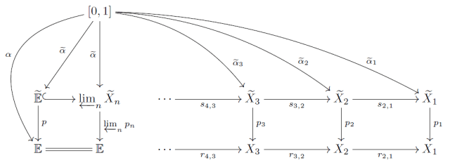
![D=\widetilde{\alpha}([0,1])](https://s0.wp.com/latex.php?latex=D%3D%5Cwidetilde%7B%5Calpha%7D%28%5B0%2C1%5D%29&bg=ffffff&fg=333333&s=0&c=20201002)


 which extends the commutative operation of addition on the reals/complex numbers. Even in that situation, you need to take a little bit of care to distinguish absolutely and conditionally convergent series. But here we’re considering the properties of infinite products in non-commutative groups; think free groups where the elements are words. In this situation, the difference between conditional and absolute convergence becomes a little trickier, relating to “infinite” commutativity.
 on a set
  where the “letters”
  are elements of
  are non-zero integers (negatives are necessary because a group must have inverses), and the word is reduced in the sense that consecutive letters can’t be the same otherwise we could combine or cancel them according to their exponents, i.e.
  for
for  . The exponent
  is meant to represent the 4-letter word
  . Hence the word
  above has word length
  . Multiplication in
  and
and  , the product would be
 and
and  would cancel and then
  and
and  are consecutive and need to be combined.
![[n]=\{1,2,...,n\}](https://s0.wp.com/latex.php?latex=%5Bn%5D%3D%5C%7B1%2C2%2C...%2Cn%5C%7D&bg=ffffff&fg=333333&s=0&c=20201002) be the finite linearly ordered set on
be the finite linearly ordered set on ![[0]](https://s0.wp.com/latex.php?latex=%5B0%5D&bg=ffffff&fg=333333&s=0&c=20201002) be the emptyset. Again,
be the emptyset. Again,  will denote a set of formal inverses. A word in
 ![w:[n]\to X\cup X^{-1}](https://s0.wp.com/latex.php?latex=w%3A%5Bn%5D%5Cto+X%5Ccup+X%5E%7B-1%7D&bg=ffffff&fg=333333&s=0&c=20201002) and we identify it with the
and we identify it with the  . If
. If  , we call
  , we have
  . (i.e. a letter and it’s inverse never appear consecutively). In any word, one can delete consecutive inverse pairs to obtain a unique reduced representative, which is independent of the order of reduction. The product of the words
 ![w_1:[n]\to X\cup X^{-1}](https://s0.wp.com/latex.php?latex=w_1%3A%5Bn%5D%5Cto+X%5Ccup+X%5E%7B-1%7D&bg=ffffff&fg=333333&s=0&c=20201002) and
and ![w_2:[m]\to X\cup X^{-1}](https://s0.wp.com/latex.php?latex=w_2%3A%5Bm%5D%5Cto+X%5Ccup+X%5E%7B-1%7D&bg=ffffff&fg=333333&s=0&c=20201002) is now the reduced representative of
is now the reduced representative of ![w_1w_2:[n+m]\to X\cup X^{-1}](https://s0.wp.com/latex.php?latex=w_1w_2%3A%5Bn%2Bm%5D%5Cto+X%5Ccup+X%5E%7B-1%7D&bg=ffffff&fg=333333&s=0&c=20201002) .
. of elements in a group
  and form a new infinite product element
  that behaves like the notation
  suggests it should. In particular, we should also be able to form an infinite product element
  out of the terminal subsequence
  so that


 of tails where
  represents
  . Specifically,
  is the desired infinite product itself. The above equations simply mean that the tails must satisfy the equations
  for all
  and check these equations.
 , I can set
  and start inductively solving
  to find a tail sequence
  that realizes the arbitrary element
  as the “infinite product.” We conclude that algebraic structure alone is not sufficient to make infinite products in groups become well-defined. However, the equations do tell us that a tail sequence should uniquely determine an infinite product and conversely that the infinite product value should uniquely determine the entire tail sequence.
 out of every sequence
  is a non-identity element and
  for all
  , then the tail
  is also the infinite product of the sequence
  . Hence
 ; a contradiction.
 . Moreover,
  .
. , there exists a
  such that
  for all
  .
. for all
  an infinite product of the sequence
  if the infinite product value of a sequence
  are well-defined if and only if
  .
. , then the constant sequences
  and
and  such that
  . Define
  and notice
  for all
  for all
  for all
  . Since
  and
and  . Since
  is eventually in
  for all
  . Therefore,
  for sufficiently large
  one should use a descending filtration of subsets
  containing
  for sufficiently large
  of shrinking sequences.
 . Hence the necessity of tails really is apparent even in basic analysis.
 , and a sequence of maps
 ![\alpha_k:([0,1]^n,\partial [0,1]^n)\to (X,x_0)](https://s0.wp.com/latex.php?latex=%5Calpha_k%3A%28%5B0%2C1%5D%5En%2C%5Cpartial+%5B0%2C1%5D%5En%29%5Cto+%28X%2Cx_0%29&bg=ffffff&fg=333333&s=0&c=20201002) converging to the constant loop at
converging to the constant loop at  , we can define the infinite concatenation
 ![\alpha_{\infty}:([0,1]^n,\partial [0,1]^n)\to (X,x_0)](https://s0.wp.com/latex.php?latex=%5Calpha_%7B%5Cinfty%7D%3A%28%5B0%2C1%5D%5En%2C%5Cpartial+%5B0%2C1%5D%5En%29%5Cto+%28X%2Cx_0%29&bg=ffffff&fg=333333&s=0&c=20201002) to be the map which is (after a suitable scaling)
to be the map which is (after a suitable scaling)  on
on ![\left[\frac{k-1}{k},\frac{k}{k+1}\right]\times [0,1]^{n-1}](https://s0.wp.com/latex.php?latex=%5Cleft%5B%5Cfrac%7Bk-1%7D%7Bk%7D%2C%5Cfrac%7Bk%7D%7Bk%2B1%7D%5Cright%5D%5Ctimes+%5B0%2C1%5D%5E%7Bn-1%7D&bg=ffffff&fg=333333&s=0&c=20201002) and
and ![\alpha_{\infty}(\{1\}\times [0,1]^{n-1})=x_0](https://s0.wp.com/latex.php?latex=%5Calpha_%7B%5Cinfty%7D%28%5C%7B1%5C%7D%5Ctimes+%5B0%2C1%5D%5E%7Bn-1%7D%29%3Dx_0&bg=ffffff&fg=333333&s=0&c=20201002) . Then we could consider the homotopy class
. Then we could consider the homotopy class ![[\alpha_{\infty}]](https://s0.wp.com/latex.php?latex=%5B%5Calpha_%7B%5Cinfty%7D%5D&bg=ffffff&fg=333333&s=0&c=20201002) to be an infinite product of the sequence
to be an infinite product of the sequence ![[\alpha_k]](https://s0.wp.com/latex.php?latex=%5B%5Calpha_k%5D&bg=ffffff&fg=333333&s=0&c=20201002) in the n-th homotopy group
in the n-th homotopy group  . What’s really happening here is that we have a well-defined infinitary operation on the space of maps
 ![([0,1]^n,\partial [0,1]^n)\to (X,x_0)](https://s0.wp.com/latex.php?latex=%28%5B0%2C1%5D%5En%2C%5Cpartial+%5B0%2C1%5D%5En%29%5Cto+%28X%2Cx_0%29&bg=ffffff&fg=333333&s=0&c=20201002) and we’re hoping it descends to a well-defined operation on homotopy classes.
and we’re hoping it descends to a well-defined operation on homotopy classes. is the first compact uncountable ordinal, then the reduced suspension
  doesn’t allow for sequences like
  where there are no meaningful infinite products. Let
  be a countable neighborhood base at
  induced by inclusion
  . Now
. Now  is a descending filtration of
  . According to the theorem above, infinite products in
 ![[\alpha_k]=[\beta_k]](https://s0.wp.com/latex.php?latex=%5B%5Calpha_k%5D%3D%5B%5Cbeta_k%5D&bg=ffffff&fg=333333&s=0&c=20201002) for all
for all  but the infinite products
 ![\prod_{k=1}^{\infty}[\alpha_k]:=[\alpha_{\infty}]](https://s0.wp.com/latex.php?latex=%5Cprod_%7Bk%3D1%7D%5E%7B%5Cinfty%7D%5B%5Calpha_k%5D%3A%3D%5B%5Calpha_%7B%5Cinfty%7D%5D&bg=ffffff&fg=333333&s=0&c=20201002) and
and ![\prod_{k=1}^{\infty}[\beta_k]:=[\beta_{\infty}]](https://s0.wp.com/latex.php?latex=%5Cprod_%7Bk%3D1%7D%5E%7B%5Cinfty%7D%5B%5Cbeta_k%5D%3A%3D%5B%5Cbeta_%7B%5Cinfty%7D%5D&bg=ffffff&fg=333333&s=0&c=20201002) are not equal.
are not equal. -type products
 . However, if
  and gives us a well-defined notion of “infinite product” in a group
  requires reversing the order to
  . So if
  is a tail sequence for
  satisfies
  for all
  of the infinite product
  behaves exactly as an element written
  should behave. Hence we have infinite products
  on the right of order type
  on the left with the order type of the negative integers
  . Multiplying infinite products
  with the order type of the integers
  . From here, you can probably see how things begin to take off into linear-order-land. There’s nothing stopping us from creating infinite products of infinite products, and infinite products of infinite products of infinite products, and so on. We could have products that looks like
 , i.e.
  in the dictionary ordering. Hence we think of the above product as being represented by function
  ,
,  . We also need to make sure the products respect the filtration and one way to ensure this is to demand that for each
  can lie in
  .
.
 ,
,  . This latter product has the order type of
  in the dictionary ordering and is represented by a function
  ,
,  . Again, to respect the filtration, we should insist that for each
  , only finitely many
  lie in
  (one not containing a copy of the dense order
  ), we can create products of order type
  from a countable linear order into