This is the sequel to Shape injectivity of the earring space (Part I)
We’re on our way to proving the canonical homomorphism  from the earring group to the inverse limit of free groups is injective. Part I was mostly dedicated to proving that an inverse limit of trees contains no simple closed curve. I’d like to reiterate here that the proof I’m detailing is almost completely self-contained; we’ll need to review two classical results from Continuum Theory; both are proved in Sam Nadler’s very readable book [2].
As a bonus, I hope you’ll find, in this two-part post, another excellent example of why general mathematical theory is worth developing. Our proof uses several existence/structure theorems that, by themselves, don’t tell you how to do anything practical. However, they can be used together to prove the Shape Injectivity Theorem, which does provide something concrete: a practical way to study and do calculations in the most fundamental class of groups with non-commutative infinite products.
Peano Continua and Dendrites
Definition: A Peano continuum is a connected, locally path-connected, compact metrizable space.
The following theorem is an important characterization of Peano continua (See [Nadler, 8.18]) that every topologist should keep in their back pocket.
Hahn-Mazurkiewicz Theorem: A space  is a Peano continuum if and only if it is Hausdorff and there is a continuous surjection
 ![[0,1]\to X](https://s0.wp.com/latex.php?latex=%5B0%2C1%5D%5Cto+X&bg=ffffff&fg=333333&s=0&c=20201002) .
.
Definition: A dendrite is a Peano continuum containing no simple closed curve.
Based on an early lemma from Part I, we could define a dendrite to be a uniquely arc-wise connected Peano continuum. Intuitively, a dendrite is a one-dimensional Peano continuum without any holes.
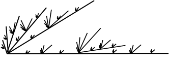
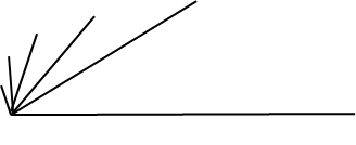
First, consider the “arc hedgehog” space  which is a one-point union of a shrinking sequence of arcs of length
  . This space came up in an early post about the category of locally path-connected spaces. It’s easy to see that is uniquely arc-wise connected and is therefore a dendrite.

The arc hedgehog dendrite
How complicated can a dendrite be? Start with , which has a single branch point, meaning that if we delete it, the subspace left has at least 3 components. At the midpoint  of a segment of length , attach a copy of scaled to have diameter
  . Continue the process inductively in a dense pattern to construct the following dendrite called Wazewski’s Universal Dendrite.
Wazewski’s Universal Dendrite
Notice there are no open sets in the Universal Dendrite homeomorphic to an open interval. In fact, this dendrite contains a homeomorphic copy of every dendrite as a retract. Hence, as far as dendrites go, the universal dendrite is as complicated as a dendrite can be.
The second result we’ll need from continuum theory provides us with a convenient way of writing down a dendrite as an inverse limit.
Dendrite Structure Theorem [Nadler, 10.27]: Every dendrite is homeomorphic to the inverse limit of a sequence of tree’s  where
where ![T_1=[0,1]](https://s0.wp.com/latex.php?latex=T_1%3D%5B0%2C1%5D&bg=ffffff&fg=333333&s=0&c=20201002) ,
,  is an arc, and the bonding retractions
  collapse the arc to the attachment point
  .
.
This structure theorem just tells you that some inverse system exists, it doesn’t help you find one. It’s a good exercise to figure out how you’d actually realize some dendrites as inverse limits of trees in the specified fashion. I recommend working out the arc-hedgehog space and Wazewski’s Universal Dendrite as examples. Hint: create an inverse system by enumerating the arcs by size.
We’ll use the Dendrite Structure Theorem to prove the last technical ingredient we’ll need. It appears as Exercise 10.51 in [2] and, I believe, is usually attributed to Borsuk.
Theorem: Dendrites are contractible.
Originally, I had posted an inverse-limit proof that uses the Dendrite Structure Theorem here that was not correct. At some point, I’ll come back and post a corrected proof using inverse limits. There is also a way to prove dendrites are contractible using metrization theory. Every dendrite  admits a metric
  such that for all distinct
  , there is an isometric embedding
 ![i_{x,y}:[0,d(x,y)]\to D](https://s0.wp.com/latex.php?latex=i_%7Bx%2Cy%7D%3A%5B0%2Cd%28x%2Cy%29%5D%5Cto+D&bg=ffffff&fg=333333&s=0&c=20201002) onto the unique arc with endpoints
onto the unique arc with endpoints  and
and  (this is called an
  -tree metric). We fix
  and define contraction
 ![H:D\times [0,1]\to D](https://s0.wp.com/latex.php?latex=H%3AD%5Ctimes+%5B0%2C1%5D%5Cto+D&bg=ffffff&fg=333333&s=0&c=20201002) so that
so that  . Then $H(x,1)=x$, $H(x,0)=v$ and one can show without too much difficulty that
  is continuous.
Proof of the Shape Injectivity Theorem
Finally, we get to the point. Ok, remember the homomorphism  ,
, ![\phi([\alpha])=([r_1\circ\alpha],[r_2\circ\alpha],\dots)](https://s0.wp.com/latex.php?latex=%5Cphi%28%5B%5Calpha%5D%29%3D%28%5Br_1%5Ccirc%5Calpha%5D%2C%5Br_2%5Ccirc%5Calpha%5D%2C%5Cdots%29&bg=ffffff&fg=333333&s=0&c=20201002) from the first post? To show it’s injective, we’ll show
from the first post? To show it’s injective, we’ll show  is trivial. Suppose that
 ![\alpha:[0,1]\to \mathbb{E}](https://s0.wp.com/latex.php?latex=%5Calpha%3A%5B0%2C1%5D%5Cto+%5Cmathbb%7BE%7D&bg=ffffff&fg=333333&s=0&c=20201002) is a loop based at
is a loop based at  such that
 ![r_n\circ\alpha:[0,1]\to X_n](https://s0.wp.com/latex.php?latex=r_n%5Ccirc%5Calpha%3A%5B0%2C1%5D%5Cto+X_n&bg=ffffff&fg=333333&s=0&c=20201002) is null-homotopic for every
is null-homotopic for every  . We must show that
  is null-homotopic in
  .
.
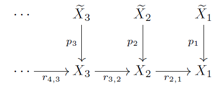
Each space  is a wedge of circles and therefore has a universal covering space
  , which is an infinite tree. In particular, is the Caley graph of
  . Let
. Let  be the universal covering map.
After making a choice of vertex basepoints  , notice that the map
  from the simply connected covering space has a unique lift
  such that
  .
.

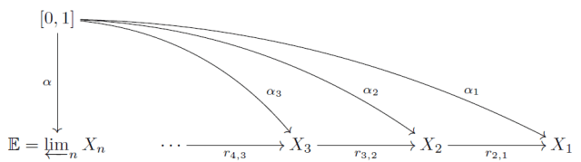
This gives us an inverse system of based covering maps.
Consider the inverse limit  . There are two things to be wary of: 1. the inverse limit of path-connected spaces is not always path-connected and 2. and an inverse limit of covering maps is not usually a covering map. But these general failures are not a deal-breaker in our situation.
First, pick a path component of  . Specifically, take
  to be the path component containing the basepoint
  . Let
. Let  be the restriction of
  .
.

While the map  is not a traditional covering map, it is surjective and it enjoys all of the usual lifting properties of a covering map. It is a kind of “generalized covering map.” Also, the space is not a dendrite. In fact, with the subspace topology inherited from the inverse limit, it’s not even locally path connected. However, if you apply the locally path-connected coreflection to it, the result is a true generalized universal covering in the sense of [1]. For our purposes, we only need to recognize that is sitting inside an inverse limit of trees.
Lemma: is uniquely arc-wise connected. In particular, it contains no simple closed curves.
Proof. The main theorem proved in Part I is that the limit of an inverse system of trees contains no simple closed curves. Since each covering space is a tree, this theorem applies and we conclude that contains no simple closed curve. In particular, the path component contains no simple closed curve. 
Recall that is a loop based at such that, for all , the projection loop ![\alpha_n=r_n\circ\alpha:[0,1]\to X_n](https://s0.wp.com/latex.php?latex=%5Calpha_n%3Dr_n%5Ccirc%5Calpha%3A%5B0%2C1%5D%5Cto+X_n&bg=ffffff&fg=333333&s=0&c=20201002) onto the wedge of n-circles is null-homotopic in . We are looking to build a null-homotopy of from a choice of null-homotopies of the approximating loops
onto the wedge of n-circles is null-homotopic in . We are looking to build a null-homotopy of from a choice of null-homotopies of the approximating loops  despite the fact that these null-homotopies might seem completely unrelated.
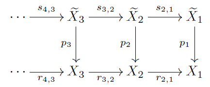
Let ![\widetilde{\alpha}_n:([0,1],0)\to (\widetilde{X}_n,\widetilde{x}_n)](https://s0.wp.com/latex.php?latex=%5Cwidetilde%7B%5Calpha%7D_n%3A%28%5B0%2C1%5D%2C0%29%5Cto+%28%5Cwidetilde%7BX%7D_n%2C%5Cwidetilde%7Bx%7D_n%29&bg=ffffff&fg=333333&s=0&c=20201002) be the unique lift of
be the unique lift of  starting at
  , i.e. so that
  . Since is null-homotopic in , it must be the case that each is actually a loop based at
  . The diagram below shows the following equalities hold:

Since  preserves the basepoints (by construction) and is the unique lift of starting at , the equality above tells us that
  . This means the lifted loops
  agree with the bonding maps of the covering space inverse system. The universal property of the top inverse system hands us a unique loop
 ![\widetilde{\alpha}:[0,1]\to \varprojlim_{n}\widetilde{X}_n](https://s0.wp.com/latex.php?latex=%5Cwidetilde%7B%5Calpha%7D%3A%5B0%2C1%5D%5Cto+%5Cvarprojlim_%7Bn%7D%5Cwidetilde%7BX%7D_n&bg=ffffff&fg=333333&s=0&c=20201002) based at
based at  satisfying
  .
.
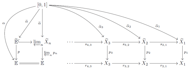
Now ![D=\widetilde{\alpha}([0,1])](https://s0.wp.com/latex.php?latex=D%3D%5Cwidetilde%7B%5Calpha%7D%28%5B0%2C1%5D%29&bg=ffffff&fg=333333&s=0&c=20201002) is the continuous image of
is the continuous image of ![[0,1]](https://s0.wp.com/latex.php?latex=%5B0%2C1%5D&bg=ffffff&fg=333333&s=0&c=20201002) in a Hausdorff space so, by the Hahn-Mazurkiewicz Theorem, is a Peano continuum. Moreover, since is path connected and contains , we have
in a Hausdorff space so, by the Hahn-Mazurkiewicz Theorem, is a Peano continuum. Moreover, since is path connected and contains , we have  . Since contains no simple closed curves, neither does
  Therefore, is a dendrite. Finally, we apply the theorem (from earlier in this post) all dendrites are contractible. Since
  factors through a contractible space, it is null-homotopic in . We conclude that
  is null-homotopic in . This completes the proof that is trivial.
Concluding Thoughts
Where did the null-homotopy of come from? It would have required a super-technical effort to build an explicit homotopy so we passed the hard work off to Borsuk’s Theorem that dendrites are contractible. Using Part I and the Hahn-Mazurkiewicz Theorem, we could say that the space is a dendrite in the first place. Then follow any proof of the contractibility of dendrites to finish the job.
Notice that we basically didn’t use anything specific about the earring space except that the universal covers of the approximating spaces are trees! So we could replace the earring with any inverse limit of graphs and the same proof would go through. So actually, we proved:
One-Dimensional Shape Injectivity Theorem: If  is an inverse limit of based graphs
  , then the canonical induced homomorphism
  to the inverse limit of free groups is injective.
For example, any one-dimensional Peano continuum (including the Menger Curve and Sierpinski Carpet) can be written as the inverse limit of finite graphs and falls within the scope of this useful theorem.
If you feel comfortable with the end of the proof, then you can also prove as a quick exercise that every inverse limit of graphs is aspherical, i.e. has trivial higher homotopy groups!
References.
[1] H. Fischer and A. Zastrow, Generalized universal covering spaces and the shape group, Fund. Math. 197 (2007) 167-196.
[2] S. Nadler, Continuum Theory: An Introduction, Chapman & Hall/CRC Pure and Applied Mathematics. 1992.


Pingback: Shape injectivity of the Hawaiian earring Part I | Wild Topology
Pingback: Homotopically Reduced Paths: Part I | Wild Topology
Pingback: Homotopically Reduced Paths (Part III) | Wild Topology