Homotopically Reduced Paths (Part III)

In this last post about reduced paths, I’m going to work through the details of one of the most useful results in wild topology. Writing this post helped me work out my own way of proving this result and hopefully will help bring together some ideas from the literature in a unique way in a way that is helpful to folks trying to learn about some of the techniques of the field.

Unique Reduced Path Theorem: If $X$ is a one-dimensional Hausdorff space, then every path $\alpha:[0,1]\to X$ is path-homotopic to a reduced path $\beta:[0,1]\to X$ that is unique up to reparameterization. Moreover, the homotopy between $\alpha$ and $\beta$ has image in $Im(\alpha)$ .

Although stated a little differently, this was basically proven in [2]. The contemporary version appears in [1]. This theorem changed the game for me. Instead of using inverse limits all of the time, this allowed me to understand and prove things using order theory and unique reduced representatives.

First, it might be helpful to give more explanation of the statement itself.

What does one-dimensional mean? Actually, you can use any of the three standard notions of dimension (Lebesgue covering, small inductive, or large inductive) and this theorem would still be true. Generally, Lebesgue covering dimension is the typical choice.
Recall from Part I that a path $\beta:[0,1]\to X$ being reduced means that $\beta$ has no null-homotopic subloops, i.e. there is no $[a,b]\subseteq [0,1]$ such that $\beta|_{[a,b]}$ is a null-homotopic loop.
What does “unique up to reparameterization” mean? A path $\beta:[a,b]\to X$ is a reparameterization of a path $\gamma:[c,d]\to X$ if there is an increasing homeomorphism $h:[c,d]\to [a,b]$ such that $\beta\circ h=\gamma$ . I use the notation $\beta\equiv\gamma$ when this occurs. Reparameterization is an equivalence relation on the set of paths in a space. So “unique up to reparameterization” means that if $\alpha$ and $\beta$ are homotopic reduced paths in a 1-dim. space, then $\alpha\equiv \beta$ .
The last statement of the theorem implies that deforming $\alpha$ to its reduced representative only requires deleting portions of $\alpha$ . As a special case, if $\alpha$ is a null-homotopic loop, then it contracts in its own image.

One-dimensional Peano continua

We need to dive into some terminology and “well-known” results from General Topology here. I’ve used these terms and results before but here’s a reminder:

An arc (respectively, simple closed curve) in a space $X$ is a subspace of $X$ that is homeomorphic to $[0,1]$ (respectively, $S^1$ ). If $h:[0,1]\to X$ is an embedding onto the arc $A=h([0,1])$ , we call $h(0)$ and $h(1)$ the endpoints of the arc. Notice that an “arc” is technically not the same thing as an embedding $[0,1]\to X$ . Rather an arc is the image of such an embedding with the subspace topology.

A space $X$ is uniquely arcwise connected, if given any distinct $a,b\in X$ , there is a unique arc $A\subseteq X$ with endpoints $a$ and $b$ .

A Peano continuum is a connected, locally path-connected compact metric space. The Hahn-Mazurkiewicz Theorem says that a space $X$ is a Peano continuum if and only if $X$ is Hausdorff and there exists a continuous surjection $[0,1]\to X$ .

A dendrite is a Peano continuum that has no simple closed curves. I go into some of the theory of dendrites in this old post on shape injectivity. In particular, I mention a well-known structure theorem, which says that a dendrite $D$ is homeomorphic to an inverse limit $\varprojlim_{n}T_n$ of trees $T_n$ where $T_{n+1}$ is $T_n$ with a single edge attached and each bonding map $T_{n+1}\to T_n$ collapses that edge to the vertex at which it is attached. In Part II of the Shape Injectivity Post, we used this structure theorem to prove that dendrites are contractible.

To put these old posts to work here’s a theorem that I mentioned at the end of Part II.

Inverse Limit Representation Theorem [3, Theorem 1]: Every one-dimensional path-connected compact metric space $X$ can be written as an inverse limit $\varprojlim_{n}X_n$ of finite graphs $X_n$ .

In fact, this is improved a bit in [4] where it is shown that it is possible to improve a given inverse system to ensure that all bonding maps $X_{n+1}\to X_n$ map $X_{n+1}$ surjectively and simplicially onto some finite subdivision of $X_n$ .

Dendrite Factorization Lemma

The next lemma is at the heart of why we can do so much in wild one-dimensional spaces like the earring space, Menger Cube, and higher-dimensional constructions that start with one-dimensional spaces, e.g. the Harmonic Archipelago. The proof for a general space $Y$ is the same as that for loops where $Y=S^1$ so I went ahead and wrote out the general proof.

Lemma: If $X$ is a one-dimensional Hausdorff space, $Y$ is a Peano continuum, and $\alpha:Y\to X$ is a null-homotopic map based at $x_0\in X$ , then $\alpha$ factors through a dendrite, that is, there is a dendrite $D$ a map $\beta:Y\to D$ and a map $g:D\to X$ such that $\alpha=g\circ\beta$ .

Proof. Assuming that $\alpha$ is non-constant, notice that $Im(\alpha)$ is one-dimensional and Hausdorff (as a subspace of a one-dimensional Hausdorff space that admits a non-constant path). Since $Im(\alpha)$ is a Hausdorff continuous image of a Peano continuum, it is a Peano continuum by the Hahn-Mazurkiewicz Theorem. Hence, we may assume that $X=Im(\alpha)$ and that $X$ is a Peano continuum.

Using the Inverse Limit Representation Theorem, write $X=\varprojlim_{n}X_n$ with bonding maps $f_n:X_{n+1}\to X_n$ and finite graphs $X_n$ . If $g_n:X\to X_n$ are the projections, we take $x_n=g_n(x_0)$ to be the basepoints in the graphs. Let $p_n:T_n\to X_n$ be the universal covering map where $T_n$ is a tree. 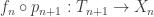As we did in Part II of the Shape Injectivity Post, once we choose basepoints $t_n\in p_{n}^{-1}(x_n)$ , the maps $f_{n}\circ p_{n+1}:T_{n+1}\to X_n$ induce unique based maps $\widetilde{f}_n:T_{n+1}\to T_n$ that give the following inverse system of covering maps.

Since $\alpha$ is null-homotopic in $X$ and each latex $p_n$ is a Hurewicz fibration, the map $\alpha_n=g_n\circ \alpha:Y\to X_n$ is null-homotopic in the graph $X_n$ and has a unique lift to a based map $\beta_n:Y\to T_n$ . These based lifts agree with the bonding maps $\widetilde{f}_n$ and give the inverse system of covering maps you see below. The universal property of inverse limits gives a unique map $\beta:Y \to \varprojlim_{n}T_n$ based at $t_0=(t_1,t_2,t_3,\dots)$ such that. $\alpha=\varprojlim_{n}p_n\circ\beta$ . In fact, Hurewicz fibrations are closed under inverse limits so $\varprojlim_{n}p_n$ is also a Hurewicz fibration!

Let $D=Im(\beta)$ . Since the inverse limit of trees $\varprojlim_{n}T_n$ is clearly Hausdorff, $D$ is a Peano continuum. Moreover, I gave a detailed proof in Part I of the Shape Injectivity Post that an inverse limit of trees contains no simple closed curves. Since $D$ is a Peano continuum with no simple closed curves, it must be a dendrite! Taking $g$ to be the restriction of $\varprojlim_{n}p_n$ to $D$ , completes the proof. $\square$

We could replace $S^1$ with any Peano continuum in the next Corollary, but I’ll try to keep it focused.

Corollary: Every null-homotopic loop $f:S^1\to X$ in a one-dimensional Hausdorff space $X$ contracts in its own image.

Proof. Suppose $\alpha:S^1\to X$ is a null-homotopic map. By the previous Lemma, we have $\alpha=f\circ\beta$ for a map $\beta:S^1\to D$ and map $f:D\to X$ where $D$ is a dendrite. Set $d_0=\beta((1,0))\in D$ . Since $D$ is contractible, there is a null-homotopy latex $H:S^1\times [0,1] \to D$ with $H(y,0)=\beta(y)$ , $H(y,1)=d_0$ . Now $f\circ H$ is a null-homotopy of $\alpha$ . $\square$

The null-homotopy $H$ in the last proof is a “free” null-homotopy but since $S^1$ is well-pointed, you could just as easily construct a basepoint-preserving homotopy.

Getting back on track, we’d like to apply the general results in Part II, which says that homotopy classes of paths will have reduced representatives if our space has well-defined transfinite $\Pi_1$ -products. So let’s make sure that happens.

Proposition: Every one-dimensional Hausdorff space has well-defined transfinite $\Pi_1$ -products.

Proof. Let $X$ be a one-dimensional Hausdorff space. Suppose $A\subseteq [0,1]$ is a closed set containing $\{0,1\}$ and $\alpha,\beta:[0,1]\to X$ are paths such that $\alpha|_{A}=\beta|_{A}$ and such that for every connected component $J$ of $[0,1]\backslash A$ , we have $\alpha|_{\overline{J}}\simeq \beta|_{\overline{J}}$ . We must show that $\alpha\simeq\beta$ . For each component $J$ of $[0,1]\backslash A$ , the loop $\alpha|_{\overline{J}}\cdot\beta|_{\overline{J}}^{-}$ is null-homotopic and therefore (by the last Corollary) contracts by a null-homotopy in $\alpha(\overline{J})\cup\beta(\overline{J})$ . In particular, there exists an endpoint-relative homotopy $H_{I}:\overline{J}\times [0,1]\to X$ , where

$H_J (s,0)=\alpha(s)$ ,
$H_J (s,1)=\beta(s)$ ,
$H_J (a,t)=\alpha(a)=\beta(a)$ and $H_J(b,t)=\alpha(b)=\beta(b)$ ,
and $Im(H_J )\subseteq \alpha(\overline{J})\cup\beta(\overline{J})$ .

We just need to put these all together! Define $H:[0,1]^2\to X$ by

$H(s,t)=\begin{cases} \alpha(s), & \text{ if }s\in A, \\ H_J(s,t), & \text{ if }s\in J\text{ for a component }J\text{ of }[0,1]\backslash A \end{cases}$

Notice that $H|_{A\times[0,1]}$ is the constant homotopy at $\alpha|_{A}=\beta|_{A}$ .

The homotopy $H$ is the constant homotopy on $A\times [0,1]$ (shaded in blue). For components $J$ of $[0,1]\backslash A$ , $H$ is defined as $H_J$ on $\overline{J}\times [0,1]$ (the white boxes).

Checking continuity of $H$ would be considered “routine” for those who make these constructions a lot so sometimes these things are skipped in the literature. But a blog is a good place to lay out the details for those who are still getting used to the proof techniques. So let’s do it!

Fix $(s,t)\in [0,1]^2$ and an open neighborhood $U$ of $H(s,t)$ in $X$ . Since each $H_J$ is continuous, $H$ is continuous at $(s,t)$ if $s\in J$ for some component $J$ of $[0,1]\backslash A$ . So we may assume $s\in A$ . Since $\alpha$ and $\beta$ are continuous at $s$ , there exists $\delta>0$ such that $\alpha([s-\delta,s+\delta])\cup \beta([s-\delta,s+\delta])\subseteq U$ . We now have $H([([s-\delta,s+\delta]\cap A)\times [0,1])=\alpha([s-\delta,s+\delta]\cap A)\subseteq U$ . If $J\subseteq [s-\delta,s+\delta]$ , then $H(\overline{J}\times [0,1])=Im(H_J)\subseteq \alpha(\overline{J})\cup\beta(\overline{J})\subseteq U$ by the definition of $H$ . What remains is to consider components $J$ having $s$ as an endpoint.

If $s$ is not an endpoint of a component of $[0,1]\backslash A$ , then we may find $c,d\in A$ such that $s\in (c,d)\subseteq [s-\delta,s+\delta]$ . If $s$ is a right endpoint of a component latex $J=(a,s)$ , then we may choose $c$ small enough so that $H((c,s]\times[0,1])=H_J((c,s]\times[0,1])\subseteq U$ (by the continuity of $H_J$ ). Similarly, if $s$ is a left endpoint of a component $J'=(s,b)$ , then we may choose $d$ small enough so that $H([s,d)\times[0,1])=H_{J'}([s,d)\times[0,1])\subseteq U$ . In any case, we can find an open interval $(c,d)$ of $s$ such that $H((c,d)\times[0,1])\subseteq U$ . $\square$

The main point of Part II, was to show that every path $\alpha$ in a Hausdorff space with well-defined transfinite $\Pi_1$ -products is path-homotopic to a reduced path. This path-homotopy was defined by “deleting” null-homotopic subloops on a maximal cancellation and therefore had image in the image of $\alpha$ . Combining this old stuff with the above proposition, it must be that every path in a one-dimensional Hausdorff space is path-homotopic to a reduced path by a homotopy that takes place in the image of that path itself. This proves the existence portion of the Unique Reduced Path Theorem as well as the last statement about the size of the homotopy required.

Uniqueness of reduced paths in one-dimensional spaces

Dendrites have their infinitely many little fingers all over this content. We’ll need them again to finish the proof of uniqueness.

Lemma: If $X$ is a one-dimensional Hausdorff space and $\alpha,\beta:[0,1]\to X$ are reduced and path-homotopic to each other, then $\alpha\equiv \beta$ , i.e. there exists an increasing homeomorphism $h:[0,1]\to [0,1]$ such that $\alpha=\beta\circ h$ .

Proof. By replacing $X$ with the image of a homotopy from $\alpha$ to $\beta$ , we may assume that $X$ is a Peano continuum. Now $\alpha\cdot\beta^{-}$ is a null-homotopic loop and so by Dendrite factorization, there exists a dendrite $D$ , a loop $\gamma:[0,1]\to D$ , and a map $f:D\to X$ such that $\alpha\cdot\beta^{-}=f\circ \gamma$ . Write $\gamma=\gamma_1\cdot \gamma_{2}^{-}$ so that $f\circ\gamma_1=\alpha$ and $f\circ\gamma_2=\beta$ . Let $d_0=\gamma_1(0)=\gamma_2(0)$ and $d_1=\gamma_1(1)=\gamma_2(1)$ . Recall that dendrites are uniquely arcwise connected and so there is a unique arc $A$ in $D$ with endpoints $d_0$ and $d_1$ . Now $\gamma_1$ is a path in $D$ from $d_0$ to $d_1$ . We check that $\gamma_1$ is injective and therefore a parameterization of $A$ . If $0\leq a<b\leq 1$ such that $\gamma_1(a)=\gamma_1(b)$ , then $(\gamma_1)|_{[a,b]}$ would be a loop. Since dendrites are contractible, $(\gamma_1)|_{[a,b]}$ is a null-homotopic loop. Then $\alpha|_{[a,b]}=f\circ(\gamma_1)|_{[a,b]}$ must also be a null-homotopic loop. However, this violates the assumption that $\alpha$ is reduced. Since $\beta$ is also reduced, applying the same argument to $\gamma_2$ shows that $\gamma_2$ also parameterizes $A$ . Since both $\gamma_1,\gamma_2:[0,1]\to A$ are homeomorphisms with the same orientation, we consider the increasing homeomorphism $h=\gamma_{2}^{-}\circ\gamma_{1}:[0,1]\to [0,1]$ . Now $\beta\circ h=f\circ\gamma_{2}\circ \gamma_{2}^{-}\circ\gamma_{1}=f\circ\gamma_1=\alpha$ , which completes the proof. $\square$ .

What’s the Takeaway?

Imagine you’ve got a based loop $\alpha:[0,1]\to X$ where $X$ is the earring space or, more amazingly, the Menger cube. The homotopy class $[\alpha]$ in the fundamental group is represented by a “tightest” loop $\beta$ that has absolutely no homotopical redundancy. Every point $\beta(t)$ is crucial to that homotopy class and the order in which those points are traced out in $X$ is completely unique.

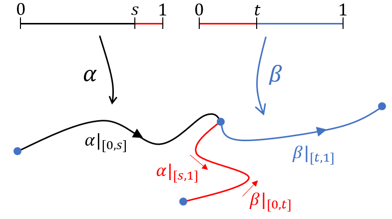
This also tells you about the operation in the fundamental groupoid $\Pi_1(X)$ too. Suppose you’ve got two composable path-homotopy classes $g,h\in \Pi_1(X)$ . Write $g=[\alpha]$ and $h=[\beta]$ for reduced paths $\alpha$ and $\beta$ . Then the product $gh$ is represented by the concatenation $\alpha\cdot\beta$ . However, $\alpha\cdot\beta$ may not be reduced. But, it’s still homotopic to some reduced path $\gamma$ and that reduced representative is obtained by deleting null-homotopic subloops on a maximal cancellation. But wait! There’s only one possible way for this to happen because the entirety of $\alpha$ and $\beta$ are both reduced. A maximal cancellation of $\alpha\cdot\beta$ can only contain one interval, which must contain the concatenation point $1/2$ . Hence, there exists $0<s<1$ and $0<t<1$ such that $\alpha|_{[s,1]}\simeq \beta|_{[0,t]}^{-}$ . There’s more! If a path is reduced, then all of its subpaths are reduced too. Since $\alpha|_{[s,1]}$ and $\beta|_{[0,t]}^{-}$ are homotopic reduced paths, which means they are actually reparameterizations of each other.

In one-dimensional spaces, a concatenation $\alpha\cdot\beta$ of reduced paths can only reduce by a cancelation of a terminal subpath of $\alpha$ and an initial subpath of $\beta$ . Each of these cancelling subpaths (in red) must be a reparameterization of the reverse of the other. The resulting reduced path is shown in black and blue is the unique reduced representative of the product $[\alpha][\beta]$ .

Theorem: Suppose $\alpha,\beta:[0,1]\to X$ are reduced paths in a one-dimensional Hausdorff space satisfying $\alpha(1)=\beta(0)$ . Then either $\alpha\cdot\beta$ is reduced or there exists unique $0<s<1$ and $0<t<1$ such that $\alpha|_{[s,1]}\equiv \beta|_{[t,1]}^{-}$ and $\alpha|_{[0,s]}\cdot\beta|_{[t,1]}$ is a reduced path representing $[\alpha][\beta]$ .

[1] J.W. Cannon, G.R. Conner, On the fundamental groups of one-dimensional spaces, Topology Appl. 153 (2006) 2648–2672.

[2] M.L. Curtis, M.K. Fort, Jr., The fundamental group of one-dimensional spaces, Proc. Amer. Math. Soc. 10 (1959) 140–148.

[3] Mardešic, S., Segal, J., $\epsilon$ –Mappings onto polyhedra. Trans. Am. Math. Soc. 109, 146–164 (1963)

[4] Rogers, J.W. Jr., Inverse limits on graphs and monotone mappings. Trans. Am. Math. Soc. 176, 215–225 (1973)