What does “wildness” really refer to?
I’ll post about higher dimensional wildness soon but to avoid getting too general, I’m going to focus on a more specific question: what does it mean for a space to have a wild fundamental group?
If you surveyed mathematicians with this question most responses would likely say:
 has a wild fundamental group if is not semilocally simply connected.
You might get a few answers of “not locally contractible,” which is a good answer to a more general question but that would be a deflection from our current focus on  . A space can easily fail to be locally contractible but still have tame 1-dimensional homotopy. The first answer is reasonable because we often study fundamental groups using covering space theory and, assuming locally path-connectivity, has a universal (i.e. simply connected) covering space if and only if is semilocally simply connected. But does failing to be semilocally simply connected really imply that the topology interacts with the algebra of in any kind of wild fashion?
The answer is: a lot of the time, but not always.
I’ll detail both parts of this answer but I think the not always part of the answer involves some fun topology. First, some quick and possibly skip-able review:
Definition: A space is semilocally simply connected at  if there exists an open neighborhood
  such that the inclusion
  induces the trivial homomorphism
 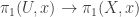 on fundamental groups. We say is semilocally simply connected if it is semilocally simply connected at all of its points.
Intuition: Despite the complicated name, the idea behind being “semilocally simply connected” is pretty straightforward. The triviality of the homomorphism simply means that every loop in based at  can be contracted in (but not necessarily in ). For instance, let
  be a cone of height
  over a circle in the xy-plane. Then the open set
  is a annular neighborhood of the base circle and is therefore homotopy equivalent to a circle. Any loop in is null homotopic in but a loop going around the base circle once is non-trivial in since you must use the top of the cone to contract it. In this case, is trivial even though
  is not.
Again, this property is a key assumption in classical covering space theory: If is path connected and locally path connected, then has a simply connected (i.e universal) covering space if and only if is semilocally simply connected.
Let’s analyze the situation where a space fails to have this property.
Topological Wildness
Definition: The topological 1-wild set of is the subspace
 .
.
Hence, for locally path-connected , the set  is precisely the topological obstruction to the existence of a universal covering space. If isn’t locally path connected, remember that we have this handy dandy tool.
Examples:
In all of the above examples, is closed in ; this is not a coincidence. Proving it’s true in general is a nice exercise to include in a course on fundamental groups.
Exercise: Prove that if is locally path-connected, then is closed in .
In fact, even in the non-locally path-connected case, something can be said.
More general exercise: Show that if  is a map from a locally path-connected space
  , then
  is closed in .
An inquisitive reader may wonder in what ways the space is a kind of homotopy invariant of . Some partial answers are published, but I promised myself not to go down the rabbit hole of writing about this yet.
What is algebraic wildness?
In particular, does  , imply that the fundamental group
  is wild?
At first glance, it seems like it might. Surely, arbitrarily small non-trivial loops are going to result in complicated algebra, right? To find out, let’s clarify what kind of property “wildness” should be for .
- It can’t be a purely group theoretic property since, by CW-approximation, every group is the fundamental group of some 2-dimensional CW-complex. I don’t care how complicated your group is or how hard the Whitehead conjecture is, the fundamental group of a CW-complex does not count as being wild.
- An algebraically “wild” fundamental group should admit at least one (possibly trivial) element that is represented by an infinite concatenation of non-contractible loops.
- It doesn’t just have to happen at the basepoint. Because of path-conjugation, wildness might occur at any point of .
Therefore, since algebraic wildness is really about the natural presence of infinitary operations like infinite sums in calculus/analysis (and in contrast with binary, trinary, or other finitary operations that come for free in ordinary groups), we’ll use the more descriptive word “infinitary” instead of “wild.”
Definition: A fundamental group  is infinitary at if there exists a loop
 ![\alpha:[0,1]\to X](https://s0.wp.com/latex.php?latex=%5Calpha%3A%5B0%2C1%5D%5Cto+X&bg=ffffff&fg=333333&s=0&c=20201002) based at , and a closed set
based at , and a closed set  with such that
 ![[0,1]\backslash C](https://s0.wp.com/latex.php?latex=%5B0%2C1%5D%5Cbackslash+C&bg=ffffff&fg=333333&s=0&c=20201002) has infinitely many components, and for each component
has infinitely many components, and for each component  of , the loop
 ![\alpha_n=\alpha|_{[a_n,b_n]}](https://s0.wp.com/latex.php?latex=%5Calpha_n%3D%5Calpha%7C_%7B%5Ba_n%2Cb_n%5D%7D&bg=ffffff&fg=333333&s=0&c=20201002) is not null-homotopic. If is not infinitary at , then we say it is finitary at . If is finitary at all points of , we say the group is finitary. If there is at least one point, where is infinitary, we say the group is infinitary.
is not null-homotopic. If is not infinitary at , then we say it is finitary at . If is finitary at all points of , we say the group is finitary. If there is at least one point, where is infinitary, we say the group is infinitary.

Two possible examples of path decompositions giving rise to an infinite product. The first example realizes an ordinary infinite product and the second case is a dense (or transfinite) product where  is the middle third Cantor set.
Equivalent but more practical definition: A fundamental group is infinitary at if and only if there exists a map  from the Hawaiian earring such that
  restricted to each circle of
  is not a null-homotopic loop.

Proof of Equivalence: If you start with the first definition, the loop satisfies  and thus induces a map
 ![f:[0,1]/C\to X](https://s0.wp.com/latex.php?latex=f%3A%5B0%2C1%5D%2FC%5Cto+X&bg=ffffff&fg=333333&s=0&c=20201002) . However, because has a countably infinite number of components,
. However, because has a countably infinite number of components, ![[0,1]/C\cong \mathbb{H}](https://s0.wp.com/latex.php?latex=%5B0%2C1%5D%2FC%5Ccong+%5Cmathbb%7BH%7D&bg=ffffff&fg=333333&s=0&c=20201002) . Moreover, each loop
. Moreover, each loop ![\alpha|_{[a,b]}](https://s0.wp.com/latex.php?latex=%5Calpha%7C_%7B%5Ba%2Cb%5D%7D&bg=ffffff&fg=333333&s=0&c=20201002) induces the restriction of to a unique circle of . Conversely, if we start with a map
induces the restriction of to a unique circle of . Conversely, if we start with a map  , let be the image of the wild point. If we take
  to be the loop which is the image of on the
  -th circle, consider the infinite concatenation
  defined as on
 ![\left[\frac{n-1}{n},\frac{n}{n+1}\right]](https://s0.wp.com/latex.php?latex=%5Cleft%5B%5Cfrac%7Bn-1%7D%7Bn%7D%2C%5Cfrac%7Bn%7D%7Bn%2B1%7D%5Cright%5D&bg=ffffff&fg=333333&s=0&c=20201002) , and
, and  . The set
  now satisfies the first definition.
Definition: The algebraic 1-wild set of a space is the subspace
 .
.
Exercise: Construct a locally path-connected space such that  is not sequentially closed.
Of course, topological 1-wildness (arbitrarily small non-contractible loops) and algebraic 1-wildness (a shrinking sequence of non-contractible loops) should feel closely related – they both involve the existence of arbitrarily small non-contractible loops at some point.
A lot of the time, they’re the same
The next theorem shows where the two kinds of wildness agree.
Theorem: If is semilocally simply connected at , then is finitary at . The converse is true if is first countable at .
Proof. Suppose is semilocally simply connected at and is a map. We must show that applied to at least one circle of is null-homotopic. Find an open neighborhood of such that every loop in based at is null-homotopic in . Write  as the usual union of circles
  of radius
  . By the continuity of , there is a neighborhood
  of
of  such that
  . Given the topology of , we may find an
  such that
  for all
  . Therefore, maps
  to a loop in , which must be null-homotopic in . This completes the first direction.
For the converse, suppose is first countable at and that is not semilocally simply connected at . Let  be a neighborhood base at . By assumption, for each
  , there is a loop
 ![\alpha_n:[0,1]\to U_n](https://s0.wp.com/latex.php?latex=%5Calpha_n%3A%5B0%2C1%5D%5Cto+U_n&bg=ffffff&fg=333333&s=0&c=20201002) based at , which is not null-homotopic in .
based at , which is not null-homotopic in .
Define a function to be on . To check the continuity of , we really only need to check the continuity of at : If is a neighborhood of , find with  . Then it is clear that
  . For
. For  find a neighborhood
  of in such that
  . Now
. Now  is a neighborhood of such that . Since is continuous an non-trivial on each circle, is infinitary.
Corollary: For any space , we have  with equality if is first countable.
So, for first countable spaces, the two notions of wildness are the same. Of course, even with some non-first countable spaces like very large CW-complexes, we still have equivalence.
This all suggests that to find a difference between topological and algebraic wildness, we need to dig into difference between nets and sequences of loops.
but not always
General Topology permits all sorts of phenomenon, including interesting spaces that are not first countable. To conclude this post, I’m going to describe a space that isn’t semilocally simply connected (and doesn’t have a universal covering space) but whose fundamental group is not wild, i.e. is finitary.
Let  be the first uncountable ordinal and
  be it’s successor, the first compact uncountable ordinal. Here, denote the maximal point of
  and we take it to be the basepoint. The key topological fact we’ll need to remember is that there does not exist any sequence in
  that converges to . Let
![X=\Sigma (\omega_1+1)=\frac{(\omega_1+1)\times [0,1]}{(\omega_1+1)\times \{0,1\}\cup\{\omega_1\}\times[0,1]}](https://s0.wp.com/latex.php?latex=X%3D%5CSigma+%28%5Comega_1%2B1%29%3D%5Cfrac%7B%28%5Comega_1%2B1%29%5Ctimes+%5B0%2C1%5D%7D%7B%28%5Comega_1%2B1%29%5Ctimes+%5C%7B0%2C1%5C%7D%5Ccup%5C%7B%5Comega_1%5C%7D%5Ctimes%5B0%2C1%5D%7D&bg=ffffff&fg=333333&s=0&c=20201002)
be the reduced suspension with canonical basepoint  . For each countable ordinal
  , the image of
 ![\{\alpha\}\times [0,1]](https://s0.wp.com/latex.php?latex=%5C%7B%5Calpha%5C%7D%5Ctimes+%5B0%2C1%5D&bg=ffffff&fg=333333&s=0&c=20201002) will result in a unique circle
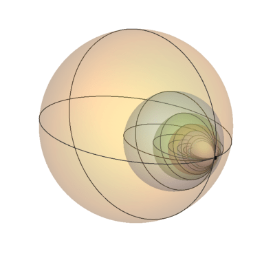
will result in a unique circle  in . These circles will all be joined at . However, the topology of this space is not the one you’d give to a wedge of CW-complexes. To help visualize this monster, consider the first convergent sequence
  in . This corresponds to the subspace
  of illustrated below as the sequence of circles
  converging to the limit circle
  .
.

From this subspace, imagine building inductively by creating larger and larger bouquet’s of circles parameterized by countable ordinals. In the limit, the circles will “converge” to in the sense that if is an open neighborhood of , then there exists a  such that
  .
.
Sorry, Not Sorry: The space is compact and it’s locally path connected at , but it’s not locally path-connected at all of its points. I take no responsibility for this. Countable limit ordinals like  are to blame. Fortunately, we’re interested in the topology around so there is no harm in sweeping this under the rug. If you’re unhappy about it, remember that you can take the locally path-connected coreflection without any loss of homotopy/homology group data. The downside to doing so is that the coreflection is not compact. So it goes.
Observation 1: is not semilocally simply connected. In particular,  .
.
Proof. Since is a quotient space of ![(\omega_1+1)\times[0,1]](https://s0.wp.com/latex.php?latex=%28%5Comega_1%2B1%29%5Ctimes%5B0%2C1%5D&bg=ffffff&fg=333333&s=0&c=20201002) and
and ![[0,1]](https://s0.wp.com/latex.php?latex=%5B0%2C1%5D&bg=ffffff&fg=333333&s=0&c=20201002) is compact, for every neighborhood of , there is a countable ordinal
is compact, for every neighborhood of , there is a countable ordinal  such that . Also, retracts onto each circle . Therefore, the loop traversing
  is contained in and is not contractible in . Since ordinals are totally path disconnected, every path component of
  is an open interval. Therefore, is semilocally simply connected at every point in
  .
.
Observation 2: is finitary, i.e.  .
.
Proof. Since  , if contains a point, it must be . Consider any map
  and suppose, to obtain a contradiction, that
  is not null-homotopic for each circle , of . In order for this to happen, it must be the case that, for each , there exists some arc of the circle that maps onto some circle
  .
.
In particular, we may find  such that
  is the image of the point
  in the circle (this is the point on furthest from/antipodal to ). Since
  in , the continuity of tells us that the sequence
  converges to in .
Maybe you already see the problem. Remember the one thing I said we’d need to use about ? There is no sequence of countable ordinals converging to . But if ![(\beta,\omega_1]=\{\alpha\mid \beta<\alpha\leq \omega_1\}](https://s0.wp.com/latex.php?latex=%28%5Cbeta%2C%5Comega_1%5D%3D%5C%7B%5Calpha%5Cmid+%5Cbeta%3C%5Calpha%5Cleq+%5Comega_1%5C%7D&bg=ffffff&fg=333333&s=0&c=20201002) is an arbitrary neighborhood of in , then we may take to be the open neighborhood of , which is the image of
is an arbitrary neighborhood of in , then we may take to be the open neighborhood of , which is the image of ![(\beta,\omega_1]\times [0,1]\cup (\omega_1+1)\times [0,1/3)\cup(2/3,1]](https://s0.wp.com/latex.php?latex=%28%5Cbeta%2C%5Comega_1%5D%5Ctimes+%5B0%2C1%5D%5Ccup+%28%5Comega_1%2B1%29%5Ctimes+%5B0%2C1%2F3%29%5Ccup%282%2F3%2C1%5D&bg=ffffff&fg=333333&s=0&c=20201002) in . The only way for the sequence to eventually be in is for the sequence
in . The only way for the sequence to eventually be in is for the sequence  of countable ordinals to eventually be inside
 ![(\beta,\omega_1]](https://s0.wp.com/latex.php?latex=%28%5Cbeta%2C%5Comega_1%5D&bg=ffffff&fg=333333&s=0&c=20201002) . This implies
. This implies  ; a contradiction of the topology of . Since is not in , this set must be empty.
Having made Observations 1 and 2, we conclude that even though fails to have a simply connected covering space, it’s fundamental group is completely tame. In fact, from a fundamental group perspective, it’s basically the same as an ordinary wedge of circles  , which is a CW-complex! Intuitively, the neighborhood base at is so large (more precisely, the “tightness” is so large) that shrinking sequences of loops don’t actually converge to the constant loop at and this sequential convergence is exactly what is required to have an infinitary fundamental group.
If you put together the ideas behind the proofs of Observations 1 and 2, it’s not too hard to prove the following more detailed results:
Theorem: The continuous identity function  from the ordinary (i.e. CW) wedge of circles to is a weak homotopy equivalence.
Corollary: is canonically isomorphic to the free group  on uncountably many generators.
Here’s a fun exercise I’ll leave you with.
Challenge Exercise: Construct a locally path-connected space for which is not closed.


, i.e.
.
viewed naturally as a subspace of
with the product topology. To make this identification, the
-th wedge summand is identified with the set
where
if
and
.
be the union of the first
be the retraction that collapses
to
collapsing
to
.
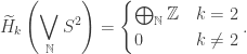
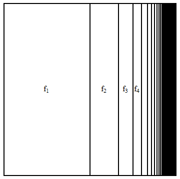
is homeomorphic to the reduced suspension
of the
-dimensional earring. By iteration, we obtain a formula similar to that for ordinary spheres:
for all
. It is important here that we use the reduced suspension and not the unreduced suspension. The undreduced suspension
is not homotopy equivalent to


![\sum_{m=1}^{\infty}[f_m]](https://s0.wp.com/latex.php?latex=%5Csum_%7Bm%3D1%7D%5E%7B%5Cinfty%7D%5Bf_m%5D&bg=ffffff&fg=333333&s=0&c=20201002)
![[f_m]\in \pi_k(\mathbb{E}_2)](https://s0.wp.com/latex.php?latex=%5Bf_m%5D%5Cin+%5Cpi_k%28%5Cmathbb%7BE%7D_2%29&bg=ffffff&fg=333333&s=0&c=20201002)
![[f_m]](https://s0.wp.com/latex.php?latex=%5Bf_m%5D&bg=ffffff&fg=333333&s=0&c=20201002)


 ,
, 


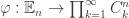

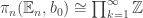


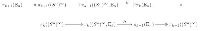
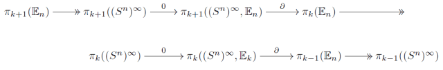
![[f_k]=a_k\in \pi_n(C_{k}^{n},b_0)](https://s0.wp.com/latex.php?latex=%5Bf_k%5D%3Da_k%5Cin+%5Cpi_n%28C_%7Bk%7D%5E%7Bn%7D%2Cb_0%29&bg=ffffff&fg=333333&s=0&c=20201002)


![f:\left[\frac{k-1}{k},\frac{k}{k+1}\right]\times I^{n-1}\to\mathbb{E}_n](https://s0.wp.com/latex.php?latex=f%3A%5Cleft%5B%5Cfrac%7Bk-1%7D%7Bk%7D%2C%5Cfrac%7Bk%7D%7Bk%2B1%7D%5Cright%5D%5Ctimes+I%5E%7Bn-1%7D%5Cto%5Cmathbb%7BE%7D_n&bg=ffffff&fg=333333&s=0&c=20201002)


![\varphi_{\#}([f])=(a_1,a_2,a_3,\dots )](https://s0.wp.com/latex.php?latex=%5Cvarphi_%7B%5C%23%7D%28%5Bf%5D%29%3D%28a_1%2Ca_2%2Ca_3%2C%5Cdots+%29&bg=ffffff&fg=333333&s=0&c=20201002)


![\varphi_{\#}([f])=(0,0,0,\dots)](https://s0.wp.com/latex.php?latex=%5Cvarphi_%7B%5C%23%7D%28%5Bf%5D%29%3D%280%2C0%2C0%2C%5Cdots%29&bg=ffffff&fg=333333&s=0&c=20201002)


![s\in \left[\frac{k-1}{k},\frac{k}{k+1}\right]](https://s0.wp.com/latex.php?latex=s%5Cin+%5Cleft%5B%5Cfrac%7Bk-1%7D%7Bk%7D%2C%5Cfrac%7Bk%7D%7Bk%2B1%7D%5Cright%5D&bg=ffffff&fg=333333&s=0&c=20201002)


 if and only if
  is a singleton.
![\frac{1}{2^{n-1}}\in [0,1]](https://s0.wp.com/latex.php?latex=%5Cfrac%7B1%7D%7B2%5E%7Bn-1%7D%7D%5Cin+%5B0%2C1%5D&bg=ffffff&fg=333333&s=0&c=20201002) . The wild set is
. The wild set is  , which is not discrete.
 Notice that this space is wild at
  is the dyadic arc-space pictured below as the union of the base-arc
 ![B=[0,1]\times \{0\}](https://s0.wp.com/latex.php?latex=B%3D%5B0%2C1%5D%5Ctimes+%5C%7B0%5C%7D&bg=ffffff&fg=333333&s=0&c=20201002) and countably many semi-circles, then
and countably many semi-circles, then  is an interval and thus has uncountably many points.

 ! Examples include the Menger Curve, Sierpinski Triangle, and Sierpinski Carpet.