The main complicating factor with the quotient topology on the fundamental group is that it often fails to be a topological group. More generally, if is a topological monoid and the quotient space is group by a relation that preserves the operation, then need not be a topological group. From one viewpoint, this could be considered a disappointing fact. So what causes this failure to happen? It turns out that this is a fairly deep topological question that I don’t have a complete answer too. It is partially due to some issues with the general topological category.
At this point, some folks may be inclined to point out that this failure doesn’t occur if one works internal to some “nicer” category like the category of k-spaces. This is a fair point. I agree that there are many situations in which the k-space category is more suitable and that one can obtain a group-object for in k-spaces. However, most folks who are adamant about forcing things into a “convenient” category (typically in AT) are uncomfortable outside of such categories and are not used to dealing with objects where the actual topology matters. To insist that a convenient coreflection is the only reasonable “fix” is short-sighted and closes the door to good mathematics. It turns out that forcing things into the k-space category loses too much information that is actually important to topologized fundamental groups and what they are good at detecting. If I had only stuck with k-spaces and been closed off to considering more challenging topological options, I wouldn’t have come up with the mathematics for what has (weirdly) become my most popular paper and led to surprising applications in topological group theory.
In this post, I’m going to talk about the actual “topological fix” to the quotient topology of . We’re going to decide if there exists a functorial topology on that gives a topological group while retaining as much of the original information of the quotient topology as possible. Along the way, we’ll explore some interesting mathematical structures and categorical topology.
Let’s approach this from a very general viewpoint. Say I have a group with identity element and some topology on . The pair might already be a topological group. If so, great! Leave it alone. But maybe it’s not. Maybe the group operation doesn’t interact nicely with the topology at all. Specifically, the group operation , and group inversion , are NOT assumed to be continuous. But let’s see if we can modify the topology , with minimal information loss, so that we end up with a topological group. The underlying group will be identical to the original group. It’s only the topology that’s going to change.
Let be the function . Notice that if is continuous, then inversion is continuous and group multiplication is continuous. Thus is a topological group. Conversely, if is a topological group, then is continuous.
Proposition 1. Let be a group with topology. Then the following are equivalent:
is a topological group ,
is continuous,
is a quotient map,
is a continuous open surjection.
Proof. We’ve already noted the equivalence of 1. and 2. Certainly 4 3 2 from basic topology. That 2 implies 4 is an introductory excercise in topological group theory.
Since the function tells us, in a sense, how close is to being a topological group, we can “force” it to be continuous by changing the topology of the codomain.
Given a group equipped with topology , let be the same group as but equipped with the quotient topology inherited from , i.e. so that is a quotient map. Let denote this quotient topology. Thus if and only if is open in . The identity function can be defined by and is is continuous. Hence, the topology of is coarser than that of . Also, according to Proposition 1, we have if and only if is a topological group.
So we fixed it right? Isn’t a topological group? Well…that’s not immediately clear. We’d have to check that is continuous and there does not seem to be an easy way to prove this. We only know that is continuous. Even so, it seems that we have at least moved in the right direction since we removed some open sets from to get the topology but not too many open sets.
So let’s do it again. Let be the same group as but equipped with the quotient topology inherited from with domain , i.e. so that is a quotient map. Let denote this quotient topology. Now, is a topological group if and only if . If this is the case, we may stop. If not, we try it again.
Since is a general operation we can perform for any group with any topology, we could define recursively for all where denotes the topology of . We are left with proper inclusions of topologies . This sequence will stabilize if and only if is a topological group for some . However, there is nothing promising that this will happen. So regular induction may fail us… We cry a few tears and then remember that there is, in fact, a way to continue this process to persist past infinity. This is where we are ever so grateful for
transfinite induction.
We have so far defined the induction for finite ordinals. The first infinite ordinal is . Let be the same group as but with topology . Notice that for all . The reason that this intersection makes sense (besides being a natural choice) is because the descending sequence of topologies is telling us that to end up with a topological group we must remove the open sets from and then from and so on. If we remove all of these open sets, we’re only left with those in .
Most transfinite induction arguments break into two cases – the successor ordinal case (a single step) and limit ordinal case (moving past infinitely many steps). The construction above provides a template for how to do the general transfinite induction: assume . Suppose is an ordinal and has been defined as the group with topology for every ordinal .
Successor ordinal case: Suppose for ordinal . Since is assumed to be defined, we may let , that is, the same underlying group as but with the quotient topology inherited from with domain , i.e. so that is a quotient map. Let denote the topology of .
Limit ordinal case: Suppose is a limit ordinal. Our induction hypothesis is that is defined with topology for all . Thus we let be the same group as but with the topology .
This transfinite induction results in a nested sequence of topologies all on the same group :
where I interjected some other infinite ordinals for good measure. But this sequences goes on for all ordinals.
Proposition 2: is a topological group if and only if .
Proof. If is a topological group, then is continuous and is therefore a quotient map. But quotient topologies are unique and the above construction gives that is a quotient map. Hence, . Conversely, suppse . But is continuous by construction and since we are assuming , we make this replacement in the codomain to see that is continuous. Hence, is a topological group.
This proposition tells us that the transfinite sequence of groups with topology can only stabilize if it stabilizes at a topological group. So must it stabilize?
Proposition 3: The transfinite sequence of groups with topology stabilizes at some ordinal .
Proof. Here, we have to appeal to cardinality. Suppose that the transfinite sequence of topologies never stabilizes. This means for each ordinal , is a proper subset of and all of the sets are pairwise-disjoint in the original topology . In other words, for each ordinal , we removed some at least one set as we proceeded through the induction.
But the ordinal numbers go really far…too far. If you give me any set like , there exists an ordinal number with a cardinality greater than that of . But the function , is an injection and this is a contradiction because we can’t inject into since we found so that .
Putting everything together, we get the following.
Theorem 4: The transfinite sequence of topologies stabilizes at some ordinal. In particular, the transfinite sequence of groups with topology stabilizes at a topological group, denoted .
The construction takes in a group with topology and outputs a topological group in “the most efficient way possible.” Formally, the topology of is the finest topology on the group that is (1) coarser than that of and (2) which makes the group a topological group.
Did we really need to go through all this trouble to build ? Well…there are other ways we could choose to show that topology of exists but none of them are going to have simple descriptions. Because, remember, a union of topologies need not be a topology. So we can’t build the topology from below. We really do have to carefully wittle down the topology of without removing too much information.
My bolded claim is not exactly proved yet, but this and many other things we can say about the construction become easier to prove once we show that is a functor. We’ll talk about maps in Part II.
In Part 1, I defined local n-connectivity, which says that a space has a basis of n-connected open sets, and the porperty, which says that for all , “small” maps from the -sphere contract using “small” homotopies of “relatively the same size.” The difference is subtle and often motivates the use of over local n-connectivity in metric geometry, shape theory, and wild topology.
In Part 1, I went ahead and explained the difference for paths, i.e. in dimension . In that case, the pointwise or based definitions (having the property at a given point) differ but the global properties (having the local property at all points) are equivalent: Locally 0-connected . I also pointed out some examples that showed things can get a bit wild if you don’t assume first countability. In this post, we’ll explore the higher dimensional situation, i.e. where .
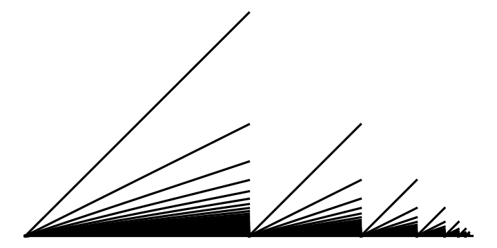
In dimension , I learned about this difference from this MathOverflow question asked back in 2019 which is really asking for an example of a space that is not locally 1-connected. Patrick Gillespie (now a PhD student at UTK and who has been a guest author on this blog) was in my topology course and asked about it. I told the class I’d offer extra credit to anyone who solved it. We had several discussions about it and Patrick came up with the space appearing in Figure 1, which I illustrated using Mathematica:
Figure 1: An example of a LC^1 space that is not locally 1-connected. Although it is not pictured, you want to imagine the large central circle filled in with a disk in this image. It becomes more difficult to see the other levels when it is included in the picture.
Construction: To build this space explicitly, the idea is to glue together a sequence of shrinking disks together in a certain way. Actually, it’s easier to visualize if you think of these disks as cones over circles. For , let be a circle with basepoint and be a loop based at that parameterizes the circle. Let be the cone over . We take the image of to be the basepoint of and we identify with the “base” of the cone, i.e. the image of . Let be the path that runs up the “spine” of the cone, that is where is the image of in .
Now, consider the wedge sum/based one-point union where the points are identified to a single wedge-point . We give the topology of a shrinking wedge determined by the following: is open if and only if is open in for all and if whenever , we have for all but finitely many (see Figure 2).
Figure 2: A shrinking one-point union of cones over the the circle. The base circles form an infinite earring and the spines of each cone runs up to the vertex.
Remark 1: is contractible by a null-homotopy that fixes the basepoint . To construct a contraction of one only need glue together null-homotopies of each cone that leaves the basepoint of (on the base circle) fixed.
Now we do some gluing. Recall that runs around the m-th base circle and runs up the m-th spine (these are both bolded in Figure 2). Let be the smallest relation on generated by for all and . The resulting quotient space the 2-dimensional Peano continuum from Figure 1 but where the large central circle is filled in by a disk or formally the cone . Let denote the quotient map. It does seem to me like this space can be embedded in although the pattern used to create Figure 1 might need to be modified a little.
Let’s make some observations about this space. Let be the image of in . This is obviously the point of interest since is locally contractible at all points in . Moreover, this space is a Peano continuum and is therefore both locally -connected at all points. Therefore, we can focus on what’s going on with loops.
Let’s once again identify with it’s image in . So still forms an infinite earring space in (that is bolded in Figure 1). Let’s also write for the image of the cone in . Note that is not a cone but is a cone where it’s vertex has been attached to one of the points on the base circle. Most importantly, we have for all .
Proposition 2: is simply connected.
Proof. By modifying standard cellular approximation methods, any given loop in based at is path-homotopic to a loop that has image in the earring space . The idea here is to start with a loop and, for all , “push it off” a given point in the interior of . This makes it easy to deformation retract the original loop to a loop with image in . But every loop lifts to a loop such that . Since is contracible, is null-homotopic. It follows that is null-homotopic.
Why isn’t locally 1-connected? Take any open neighborhood of the basepoint which does not contain the largest cone-image . Find the largest such that . Since , the loop has image in but it does not contract in because the image of a contraction of would necessarily contain . Thus is not simply connected.
Why is an space? Take any open neighborhood of the basepoint . Find the smallest such that for all . Let be a path-connected open neighborhood of such that and such that for all . Any loop in based at can be deformed onto . But the argument used to prove Proposition 2 shows any such loop is null-homotopic in the subspace , which is a subset of . Therefore, any loop in contracts in (even though it does not contract in ).
Theorem 3: There exists a 2-dimensional Peano continuum, which is and locally 0-connected but not locally 1-connected.
So the equivalence of the global properties no longer holds when . I don’t really know if there is someone I should credit this Theorem to. No doubt it was known a long time ago so I’ll call it “folklore” until I learn otherwise.
Here are some brain teasers.
Question 4: Is contractible?
Question 5: Is there a space that is not locally 1-connected at any point?
The answer to both of these questions should be “yes” but I haven’t thought too much about the details.
What about even higher dimensions? If you’re looking for an example of an space that is not locally n-connected you can mimic the above example by defining to be an -sphere instead of a circle. But the reason why the above example worked so well is because the paths are surjective – in order to contract in , you need to use all of but doing so requires that you use all of the image of , which is . Then your homotopy would have to use , which is clearly a problem. To make this same thing happen in higher dimensions (using cones), we must realize that we don’t have a canoncial way to map the spine of a cone (which is an arc) onto a higher-dimensional sphere. How do we make surjective like we did when ? If we choose to be a simple close curve, we won’t get you the kind of example we want. This is where we are thankful for space-filling curves! We can take to be any continuous surjection, i.e. space-filling curve (such maps exist due to results in Continuum Theory). Once this choice is made, pretty much all of the arguments are the same for the case work the same. This leads us to the following extension of Theorem 3.
Theorem 6: For each , there exists a n-dimensional Peano continuum, which is and locally (n-1)-connected but not locally n-connected.
I’m going to take a little break from the topologized fundamental group series for a bit. That’s a long series and a distraction might be nice. Right now, I’m going to share a little about a property I’ve been running into pretty frequently. First, a standard definition in homotopy theory.
Definition 1: A space is n-connected if is trivial for all (and some or any choice of basepoint), that is, if is path connected (0-connected) and the first through n-th homotopy groups are trivial.
Definition 2: A space is locally n-connected at if for every neighborhood of , there exists an n-connected neighborhood of such that . A space is locally n-connected if it is locally n-connected at all of its points.
Lots of spaces are locally n-connected but when you’re proving general theorems it can be difficult or impossible to actually build n-connected open sets using general methods. There is a larger class of spaces that’s often more conducive to creating and proving general results. This is the property. The fact that so many old/classic papers use this property without defining it makes me feel that it used to be more broadly used and understood. Certainly, it’s still used in metric topology and shape theory (and of course wild topology). Even though the terminology and notation are definitely established, whenever I do use it, I feel the need to define it. Personally, I feel that unless one already knows the difference, it’d be easy to see “LCn ” for the first time and assume that this means locally n-connected…you know..because of the letters.
Definition 3: A space is at if for every neighborhood of , there exists a neighborhood of such that and such that for every , every map is null-homotopic in . A space is if it is at all of its points.
The key difference between the two definitions is that in the locally n-connected definition, is chosen so that a map from a -spheres () actually can be contracted in . In the definition, is chosen so that all maps contract within the slightly larger open set . Certainly, we have:
locally n-connected at at
Examples illustrating the difference between these properties can take us to wild places so let’s work some out in low dimensions. We’ll sort out the 0-dimensional case in the remainder of this post and discuss higher dimensions in the next post.
Local 0-connectivity and
A space being locally 0-connected at a point means being locally path-connected. In this case, has a basis of path-connected open sets at . In contrast, means that is “relatively locally path-connected.” Given any small neighborhood , we can find a smaller neighborhood so that a map (where ) extends to a path . In short, any two points in can be connected by a path in but maybe not by a path in . We could be worried that this path in is too big. But remember that was already an arbitrarily small neighborhood so it is still relatively small when compared with the neighborhood . See below for an image of the two cases.
If a space is locally 0-connected at a point, V may be chosen so any map f from {-1,1} to V can be extended to a path within V (top). If the space is LC0 at a point, one may chose V but only be able to extend f to a path within U (bottom).
Because the property is a relative-size-type property, we have to stretch our brains a bit when searching for an example that distinguishes the two properties. Here’s an example of a space with a point where you have the property but not locally path connectivity.
Example 4: Consider the planar set illustrated below.
A compact planar set which is LC0 but not locally 0-connected at its rightmost point. Note that it does fail to be LC0 at all points in .
Let’s say we embed this space in the plane so the bottom arc is the closed unit interval on the x-axis. This space is locally path-connected at all points with positive y-component. It’s clearly not locally path connected at any point in but it’s less obvious what is happening at because the fans are shrinking in diameter.
First, let’s show that this space is not locally 0-connected at the rightmost point : Any neighborhood of contains one of the fan-vertices for some smallest . This is going to have to contain some of the points for but there’s no way to connect to such a point with a path in because that path would need to pass through . One can deduce from this observation that any path-connected neighborhood of must contain the entire bottom arc. So is not locally path connected at .
On the other hand, is at . A basic neighborhood of is of the form , . Given , the set is not path connected. However, any two points in can be connected by a path in because you’re allowed to move left just far enough to get to the nearest fan-vertex on the x-axis.
The above space is a compact, one-dimenisonal, planar metric space. However, it’s not a dendrite because it’s not locally connected (or even ) at several points. Actually, in Example 4, we were only able to verify that is but not locally 0-connected at because there are points besides where is not . Another way to look at it is this – in dimension , the pointwise properties are not equivalent but the global properties are. This is formalized in the next proposition.
Proposition 5: A space is if and only if it is locally 0-connected.
Proof. One direction is clear. Suppose is at all of its points. Let and be an open neighborhood of . It suffices to show that the path component of in is open in . Let , then by assumption, we can find a neighborhood of such that and such that every point can be connected to by a path in . But since is the path component of in , we have . This proves that is open.
Sequentially 0-connected spaces
For first countable spaces, it’s possible to characterize the pointwise property using the following definition.
Definition 6: A space is sequentially 0-connectedat if for every convergent sequence , there exists a path such that and . We say is sequentially 0-connected if it is sequentially 0-connected at all of its points.
I’ve been finding sequential properties like this really useful lately and there are several equivalent ways to define this property. Basically this property means that every convergent sequence extends to a continuous path. The sequentially 0-connected property is the sequential analogue of the property. I’ll justify this claim in the next theorem. In papers, I have claimed this proof is “elementary” but I don’t know of a reference for it. It will make me feel better if the proof is here.
Theorem 7: Suppose is first countable at . Then is at if and only if X is sequentially 0-connected at .
Proof. For both directions, let be a neighborhood base at . First, suppose is at and let be a convergent sequence. Find a neighborhood of such that and such that any two points in can be connected by a path in . Let . Since , it must be that . Let from to . Then every neighborhood of contains for all but finitely many . This means the infinite path-concatenation is well-defined, continuous, maps to and to .
For the other direction, suppose is not at . Then there exists open neighborhood of such that for every neighborhood of in , there exists two points in that cannot be connected by a path in . In particular, there must be some point such that and cannot be connected by a path in (if this were not the case, the previous sentence would be violated using path concatenation). Let’s assume that we have our neighborhood base . Then for every , there exists such that there is no path in from to . Note that since we are choosing points from a neighborhood base. Also, it is not possible to find a continuous path with and . Indeed, such a path would have for some and thus restrict to a path from to ; a contradiction. Since the convergent sequence cannot be extended to a path, we conclude that cannot be sequentially 0-connected at .
Since the space in Example 4 is a metric space, that example is sequentially 0-connected but not locally 0-connected. The next example is not a metric space but is more extreme. It’s topology is so large and fine that the space is sequentially 0-connected but not .
Example 8: Let be the first compact uncountable ordinal (with maximal element . We give the topology generated by singletons , and the cofinal sets . The key thing to know about is that there is no sequence of countable ordinals that converges to the maximal point . For each , attach an arc to by identifying and . Let be the resulting space with the weak topology with respect to the subspaces and , . Any sequence in that converges to eventually lies in for some fixed . All such sequences extend to a path and it follows that is sequentially 0-connected at (and thus at all of its points).
However, this space is not at . Let be the union of the images of all copies of in . Any open neighborhood of in will contain elements of but will not contain any arc . Thus there is no way to connect to the elements of by a path in or . We conclude that is not at .
The space in Example 8 is constructed by attaching arcs to the first compact uncountable ordinal (but with a modified topology).
Example 9: There is an example of a locally path-connected space, which is not sequentially 0-connected. This rather remarkable example using the Axioms of Choice is constructed by Taras Banakh in an answer to this MO question of mine. It is even -generated!
Examples 4,8, and 9 show that the pointwise-sequentially 0-connected property is comparable to neither the locally 0-connected property nor the property.
We’ll deal with the difference between local 1-connectivity and in the next post.


 porperty, which says that for all
  , “small” maps from the
  -sphere contract using “small” homotopies of “relatively the same size.” The difference is subtle and often motivates the use of
  . In that case, the pointwise or based definitions (having the property at a given point) differ but the global properties (having the local property at all points) are equivalent: Locally 0-connected
 . I also pointed out some examples that showed things can get a bit wild if you don’t assume first countability. In this post, we’ll explore the higher dimensional situation, i.e. where
  , I learned about this difference from
  space that is not locally 1-connected. Patrick Gillespie (now a PhD student at UTK and who has been a guest author on this blog) was in my topology course and asked about it. I told the class I’d offer extra credit to anyone who solved it. We had several discussions about it and Patrick came up with the space appearing in Figure 1, which I illustrated using Mathematica:
 , let
, let  be a circle with basepoint
  and
and ![\alpha_m:[0,1]\to A_m](https://s0.wp.com/latex.php?latex=%5Calpha_m%3A%5B0%2C1%5D%5Cto+A_m&bg=ffffff&fg=333333&s=0&c=20201002) be a loop based at
be a loop based at ![CA_m=[0,1]\times A_m/\{1\}\times A_m](https://s0.wp.com/latex.php?latex=CA_m%3D%5B0%2C1%5D%5Ctimes+A_m%2F%5C%7B1%5C%7D%5Ctimes+A_m&bg=ffffff&fg=333333&s=0&c=20201002) be the cone over
be the cone over  to be the basepoint of
  and we identify
  . Let
. Let ![\ell_m:[0,1]\to CA_m](https://s0.wp.com/latex.php?latex=%5Cell_m%3A%5B0%2C1%5D%5Cto+CA_m&bg=ffffff&fg=333333&s=0&c=20201002) be the path that runs up the “spine” of the cone, that is where
be the path that runs up the “spine” of the cone, that is where  is the image of
  in
in  where the points
  . We give
  the topology of a shrinking wedge determined by the following:
  is open if and only if
  is open in
  and if whenever
  , we have
  for all but finitely many
 be the smallest relation on
  for all
  and
and ![t\in[0,1]](https://s0.wp.com/latex.php?latex=t%5Cin%5B0%2C1%5D&bg=ffffff&fg=333333&s=0&c=20201002) . The resulting quotient space
. The resulting quotient space  the 2-dimensional Peano continuum
  from Figure 1 but where the large central circle is filled in by a disk or formally the cone
  . Let
. Let  denote the quotient map. It does seem to me like this space can be embedded in
  although the pattern used to create Figure 1 might need to be modified a little.
 be the image of
  . Moreover, this space is a Peano continuum and is therefore both locally
  -connected at all points. Therefore, we can focus on what’s going on with loops.
 still forms an infinite earring space in
  for the image of the cone
  for all
  with image in
 ![L:[0,1]\to \bigcup_{m\geq 1}A_m](https://s0.wp.com/latex.php?latex=L%3A%5B0%2C1%5D%5Cto+%5Cbigcup_%7Bm%5Cgeq+1%7DA_m&bg=ffffff&fg=333333&s=0&c=20201002) lifts to a loop
lifts to a loop ![L':[0,1]\to X](https://s0.wp.com/latex.php?latex=L%27%3A%5B0%2C1%5D%5Cto+X&bg=ffffff&fg=333333&s=0&c=20201002) such that
such that  . Since
  is null-homotopic. It follows that
  of the basepoint
  . Find the largest
  . Since
  , the loop
 ![\alpha_m:[0,1]\to Y](https://s0.wp.com/latex.php?latex=%5Calpha_m%3A%5B0%2C1%5D%5Cto+Y&bg=ffffff&fg=333333&s=0&c=20201002) has image in
has image in  would necessarily contain
  for all
  . Let
. Let  be a path-connected open neighborhood of
  and such that
  for all
  . Any loop in
  . But the argument used to prove Proposition 2 shows any such loop is null-homotopic in the subspace
  , which is a subset of
  , which is
  . Then your homotopy would have to use
  , which is clearly a problem. To make this same thing happen in higher dimensions (using cones), we must realize that we don’t have a canoncial way to map the spine of a cone (which is an arc) onto a higher-dimensional sphere. How do we make
  is trivial for all
  if for every neighborhood
  , there exists an n-connected neighborhood
  is null-homotopic in
  (where
  ) extends to a path
 ![[-1,1]\to U](https://s0.wp.com/latex.php?latex=%5B-1%2C1%5D%5Cto+U&bg=ffffff&fg=333333&s=0&c=20201002) . In short, any two points in
. In short, any two points in 
 .
. but it’s less obvious what is happening at
  because the fans are shrinking in diameter.
 for some smallest
  for
for  but there’s no way to connect
  . One can deduce from this observation that any path-connected neighborhood of
 ![U_n=X\cap (1-2^{-n},1]\times \mathbb{R}](https://s0.wp.com/latex.php?latex=U_n%3DX%5Ccap+%281-2%5E%7B-n%7D%2C1%5D%5Ctimes+%5Cmathbb%7BR%7D&bg=ffffff&fg=333333&s=0&c=20201002) ,
,  is not path connected. However, any two points in
  because you’re allowed to move left just far enough to get to the nearest fan-vertex on the x-axis.
 of
of  , then by assumption, we can find a neighborhood
  such that
  can be connected to
  . This proves that
  , there exists a path
 ![\alpha:[0,1]\to X](https://s0.wp.com/latex.php?latex=%5Calpha%3A%5B0%2C1%5D%5Cto+X&bg=ffffff&fg=333333&s=0&c=20201002) such that
such that  and
and  . We say
  be a neighborhood base at
  be a convergent sequence. Find a neighborhood
  of
of  and such that any two points in
  . Since
  . Let
. Let ![\beta_m:[0,1]\to U_n](https://s0.wp.com/latex.php?latex=%5Cbeta_m%3A%5B0%2C1%5D%5Cto+U_n&bg=ffffff&fg=333333&s=0&c=20201002) from
from  . Then every neighborhood of
 ![\beta_m([0,1])](https://s0.wp.com/latex.php?latex=%5Cbeta_m%28%5B0%2C1%5D%29&bg=ffffff&fg=333333&s=0&c=20201002) for all but finitely many
for all but finitely many  is well-defined, continuous, maps
  to
to  to
to  of
of  cannot be connected by a path in
 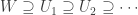 . Then for every
  such that there is no path in
  . Note that
 ![\alpha([(n-1)/n,1])\subseteq W](https://s0.wp.com/latex.php?latex=%5Calpha%28%5B%28n-1%29%2Fn%2C1%5D%29%5Csubseteq+W&bg=ffffff&fg=333333&s=0&c=20201002) for some
for some ![\alpha|_{[(n-1)/n,1]}:[(n-1)/n,1]\to W](https://s0.wp.com/latex.php?latex=%5Calpha%7C_%7B%5B%28n-1%29%2Fn%2C1%5D%7D%3A%5B%28n-1%29%2Fn%2C1%5D%5Cto+W&bg=ffffff&fg=333333&s=0&c=20201002) from
from  be the first compact uncountable ordinal (with maximal element
  . We give
  the topology generated by singletons
  ,
,  and the cofinal sets
 ![(\lambda,\omega_1]=\{\kappa\mid \kappa>\lambda\}](https://s0.wp.com/latex.php?latex=%28%5Clambda%2C%5Comega_1%5D%3D%5C%7B%5Ckappa%5Cmid+%5Ckappa%3E%5Clambda%5C%7D&bg=ffffff&fg=333333&s=0&c=20201002) . The key thing to know about
. The key thing to know about  that converges to the maximal point
 ![A_{\lambda}=[0,1]](https://s0.wp.com/latex.php?latex=A_%7B%5Clambda%7D%3D%5B0%2C1%5D&bg=ffffff&fg=333333&s=0&c=20201002) to
to  and
and  . Let
. Let  ,
,  that converges to
 ![[0,1/3)\cup (2/3,1]\subset A_{\lambda}](https://s0.wp.com/latex.php?latex=%5B0%2C1%2F3%29%5Ccup+%282%2F3%2C1%5D%5Csubset+A_%7B%5Clambda%7D&bg=ffffff&fg=333333&s=0&c=20201002) in
in 
 -generated!